Kaggle's Titanic Toy Problem with Random Forest
Kaggle proposes some interesting exercises to practice basic machine learning techniques. Among them, Titanic: Machine Learning from Disaster is a typical classification problem1 from labelled data (supervised learning). This example is very rich from an academic/pedagogic perspective. Throughout this post we present a way to address this toy problem. In particular, we show how to:
- Tinker features2. The given data set consists of a handful number of features; however many of them should be adequately modified (or combined) to improve predictability performances. We also exemplified one technique to impute missing data (especially, the data set is small, and thus we can’t afford to ignore rows with missing values)
- Select features using a basic greedy algorithm.
- Use the randomForest algorithm in R.
- Perform a simplistic grid search for finding adequate hyper parameters.
We do not pretend to give an optimal solution3. Machine learning is still very trial-and-error oriented and there is a plethora of ways that could be tried to enhance the results. There are numerous parameters that could be tuned, and current approaches resemble a form or another of a greedy algorithm (as trying all possible combination of parameters—and features—is currently intractable).
Getting a Sense of the Data Set
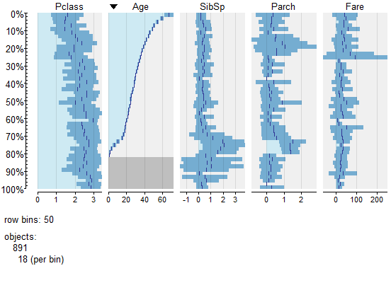

Several columns are categorical data. Tree based algorithms (such as random forest or gradient boosting machine) can usually handle those columns without problems. By contrast, other popular algorithms, such as generalized linear models or neural networks (dubbed “deep learning” nowadays) would require converting those columns to numerical (e.g., one-hot, enum or binary encoding offer possibilities to achieve this).
We can observe that the columns Age, Fare, Cabin and Embarked have some missing values. While the missing values for both Age and Cabin are consistent between the train and test sets (roughly 20% and 80% of missing values, respectively), there is only one missing Fare value in the test set and two missing Embarked values in the train set.
Features Tinkering
Remember that all manipulations made on the training set must be done on any subsequent data set for which we need to predict the outcome. Here, we have the data set X we use for crafting the machine, we have Xt for which we want to predict the outcome (i.e., the Survived column).
In this section we only present the features from which we derive non-trivial new features (e.g., we do not mention features for which we just performed minor changes; see the source code for the full details).
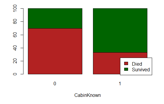
Cabin
We can observe that the chances of survival when the cabin is known are higher. Perhaps because survivors could tell their room afterwards? We add the new feature CabinKnown and drop the column Cabin (there is nearly 80% of missing values, data imputation techniques might yield rather poor outcomes).
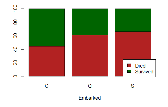
Embarked
It appears that only two passengers embarked from unknown location (in the train set, and none of them in the test set).
Those two passengers are two first-class women that survived, but it seems they have the same ticket number, the same cabin and the same fare (X[X$Embarked == "", ]). Those coincidences are rather weird; it might very well be an error in the data.
Even though the data set is small, and we already crave for more data, those two rows are overly suspicious; and thus we decide to remove them (X <- X[-which(X$Embarked == ""), ]).
Besides, we can observe two categories: The ones that embarked at Q and S have approximately the same chances of survival, which is noticeably less than the ones that embarked in C. We add the new feature EmbarkedQorS.

Ticket
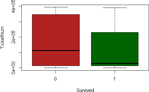
The feature Ticket seems to follow several conventions. All of them have a number, though. We extract that number and create a new feature TicketNum (and drop the Ticket column). There seem to be some outliers in those numbers. We replace those outliers with the median of the ticket numbers found in the train set (median imputation). That is very basic/naive, and we might revise this decision later on.
As odd as it can be, it appears that ticket’s numbers are correlated in some ways to the chances of survival
Name
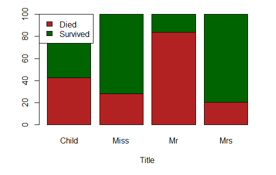
The full name of each passenger consistently shows a title. Although there are a multitude of different titles, we can aggregate them into four categories, and add the feature Title: “Mr”, “Miss” (supposedly unmarried women), “Mrs” (supposedly married women) and “Child” (it is not strictly speaking a title, but anyway…). We make the following assumptions:
- “Don”, “Rev”, “Major”, “Sir”, “Col”, “Capt”, “Jonkheer” are all “Mr”;
- “the Countess”, “Mlle”, “Ms” are all “Miss”;
- “Mme”, “Lady”, “Dona” are all “Mrs”;
- “Dr” depends on the other features Sex and SibSp to determine whether it is “Mr”, “Mrs” or “Miss” (although in 1912, it must be mostly men);
- finally, “Master” and all passengers aged below 10 are “Child”.
It appears that “Miss” and “Mrs” have more or less the same chances of survival. We add a new feature Gender that aggregates them (the name might not be the best one…). Gender and Title might be redundant. Ultimately, the features selection algorithm will pick.
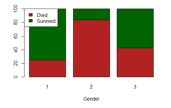
Note that we named the three levels of the categorical feature Gender, “1”, “2” and “3”. It does not matters, as the columns is categorical and not numerical.
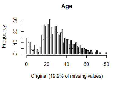
Age
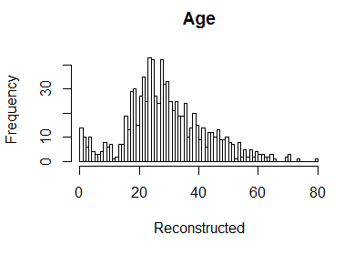
There are a non-negligible number of missing ages (about 20%). This feature seems quite important. We use data imputation to estimate the missing ages; specifically, we rely on a k-nearest neighbour imputation—other techniques could be tried, such as, e.g., imputations via bagging (see the caret package) or generalized low rank models (Udell et al., 2016).
preProcX <- preProcess(X[, -indexToIgnore],
                       method = c("knnImpute", "center", "scale"),
                       k = 8)
predictedMissingValues <- predict(preProcX, X[, -indexToIgnore])
predictedMissingValuesTest <- predict(preProcX, Xt[, -indexToIgnore])

XpredAge <- predictedMissingValues[["Age"]]
XpredAget <- predictedMissingValuesTest[["Age"]]

# we scale back the feature, because we might need the Age
# for tinkering other features
meanAge <- mean(X$Age, na.rm = TRUE)
sdAge <- sd(X$Age, na.rm = TRUE)

X$AgePred <- (XpredAge * sdAge) + meanAge
Xt$AgePred <- (XpredAget * sdAge) + meanAge
Those techniques could be regarded as—actually, they are—unsupervised learning techniques. We need to be careful not to use the test set for any preprocessing4 (data imputation is performed for the test set as well, but by using preprocessing from the train set only).
We add the new feature AgePred and drop the original one Age.
Fare
The missing Fare value in the test set is imputed using the same technique as for the missing ages imputation described above. We add the new feature FarePred and drop the original one Fare.
Parch & SibSp
We add a couple of new features from Parch and SibSp:
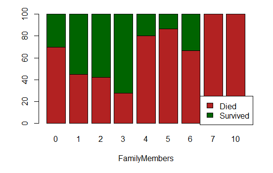
- FamilyMembers: the size of the passenger’s family (on board)
- LargeFamily: whether or not the passenger’s on-board family is large
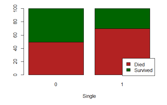
- Single: whether or not the passenger is alone
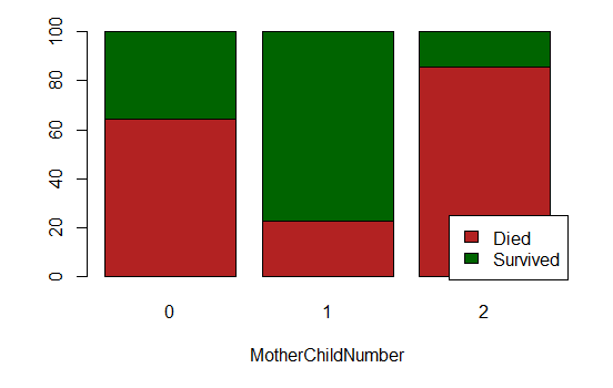
- MotherChildNumber (which uses AgePred and Title as well):
- “1” for women aged over 20 with Parch in {1, 2, 3};
- “3” for women aged over 20 with Parch strictly greater than 3;
- “0” otherwise.
Data Split
A validation set is extracted from the train set. We need a validation set (i) to assess the performance of subsets of fatures during the feature selection step, and subsequently, (ii) to select the best models out of the grid search.
One can remark that we use different proportions for (i) and (ii)—0.5 and 0.8, respectively. The rational for it lies in the fact that we do not want to pick features that are prone to overfitting (hence a larger validation set). However, a larger validation set comes at the expense of training data; so much that the resulting train set might not suffice (hence a smaller validation set during grid search).
Features Selection
We implement a forward stepwise algorithm (greedy algorithm), that does not guarantee the optimal subset of features, but that should yield a subset that performs well. To assess the performance of subsets, our implementation supports accuracy (acc), mean square error (mse), logloss and AUC (area under the ROC curve). We used AUC, because it is threshold independent and is a good metric provided that the classes to predict are not overly unbalanced (here, we have roughly 38% of survivors).
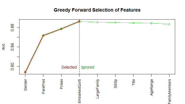
Quite surprisingly, only four features were selected: Gender, FarePred, Pclass and EmbarkedQorS.
Simplistic Grid Search
We perform a simplistic grid search (Cartesian) to find adequate hyper parameters.
hyperParams<- list ()
hyperParams$ntree <- c(50, 100, 200, 400, 500)
hyperParams$replace <- c (TRUE)
hyperParams$nodesize <- c(1, 2, 3, 4, 5)
hyperParams$maxnodes <- c(12)
hyperParams$mtry <- c(2)
...
grid <- expand.grid(hyperParams)
for(i in 1:nrow(grid)) {
  row <- grid[i, ]
  rf <- randomForest(formula, data = train,
                     ntree = row$ntree, nodesize = row$nodesize,
                     mtry = row$mtry, replace = row$replace,
                     maxnodes = row$maxnodes)

  predValid <- predict(rf, newdata = valid)
  validAcc <- mean(valid$Survived == predValid)

  oob <- mean (rf$err.rate[, "OOB"])
  ...
}
Results
Here is the sorted grid result—first decreasingly by validAcc, then increasingly by oob (we show only the “head”).
> print(head(grid, 10), row.names = FALSE)
 ntree replace nodesize maxnodes mtry    valAcc       oob index
   100    TRUE        5       12    2 0.8305085 0.2019279    22
    50    TRUE        3       12    2 0.8305085 0.2128829    11
   100    TRUE        3       12    2 0.8248588 0.2053615    12
   500    TRUE        2       12    2 0.8248588 0.2136730    10
   400    TRUE        1       12    2 0.8192090 0.2019288     4
    50    TRUE        4       12    2 0.8192090 0.2020480    16
    50    TRUE        5       12    2 0.8192090 0.2094418    21
   500    TRUE        1       12    2 0.8192090 0.2099737     5
   200    TRUE        1       12    2 0.8192090 0.2104675     3
   500    TRUE        5       12    2 0.8192090 0.2189793    25
...
Submitting the first row’s model yielded the accuracy of 0.81818 on Kaggle. ■
License and Source Code
© 2017 Loic Merckel, Apache v2 licensed. The source code is available on both Kaggle and GitHub.
References
- Udell, M., Horn, C., Zadeh, R., Boyd, S., & others. (2016). Generalized low rank models. Foundations and Trends in Machine Learning, 9(1), 1–118.
-
A similar example for regression is also available on Kaggle: House Prices: Advanced Regression Techniques. We might write a similar post on it in a short while. ↩
-
The usual term to describe the preparation of features is features engineering; however, I prefer using the term tinkering, which, I believe, offers a better description… ↩
-
The leaderboard on Kaggle shows much better results than what we obtain here—it is worth noting, though, that the Titanic’s list of passengers with their associated destiny is publicly available, and therefore it is easy to submit a solution with 100 per cent accuracy. ↩
-
One could argue that, in this particular problem, given that there will be no additional new data, the test set could be used as well in the training process… ↩