Kaggle's Titanic Toy Problem Revisited
Throughout this post we present another1 way to address the Kaggle’s toy problem Titanic: Machine Learning from Disaster. In particular, we show how to:
- Leverage unlabeled data in a supervised classification problem (a technique often referred to as semi-supervised learning).
- Use the autoencoder and deeplearning capability of the wonderful H2O framework.
Note that the method presented in this page does not propose a model that can make predictions from new data (unlike our previous approach here). The test set is extensively used during the process; it can be regarded as a label reconstruction method.
Finally, we observe fairly good results (e.g., 0.80383 on the Kaggle’s leadderboard with this source code); which is quite remarkable given the ridiculously small size of the data set (a setting usually prone to favor tree-based methods—or generalized linear model should the transformed response by the link function varies linearly with the features—over neural networks).
Features Tinkering
Feature Preparation
The features are prepared the exact same way as described in our previous post Kaggle’s Titanic Toy Problem with Random Forest (or its Kaggle version).
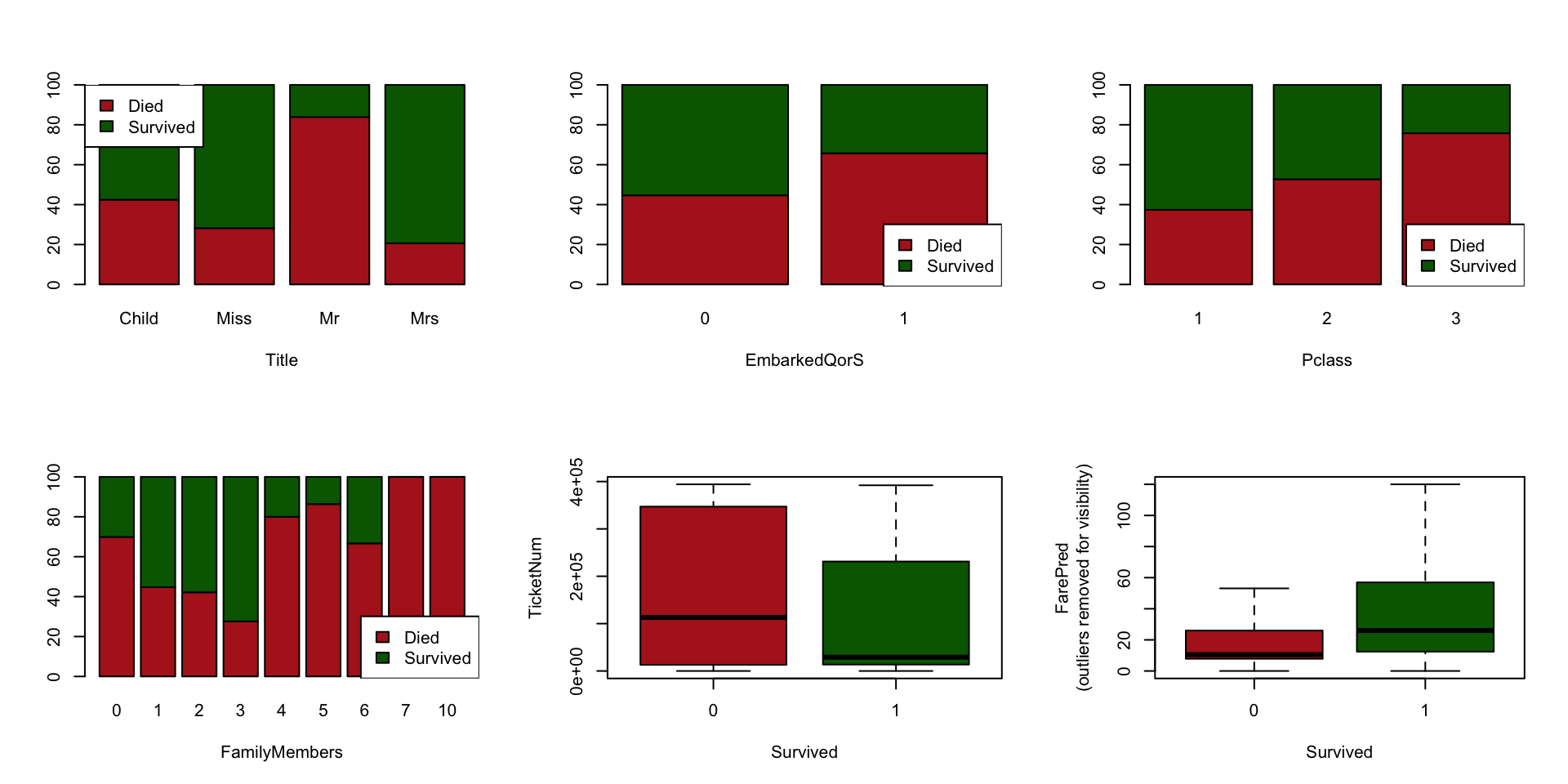
The figure below presents some charts relative to the six features we will select (see section Feature Selection).
Dealing With Categorical Variables
Unlike our previous approach relying on tree-based learning, here we use neural networks, and thus we need to encode categorical variables. The H2O framework offers, out-of-the-box, several of the popular techniques to achieve such an encoding: one-hot, binary, enumeration (label)—plus some other methods, see here for a full description.
Enum encoding is often a poor choice, unless there exist a meaningful order relationship between the categories. If ordering categories does not make sense—e.g., the Title feature consists of four categories: Child, Miss, Mr and Mrs—then other encodings might constitute wiser options.
Binary encoding makes sense when the number of categories is large; it typically adds 32 columns per categorical variable—and therefore one-hot encoding appears the right choice when the number of categories is less than 32.
In our selected subset of features (see section Feature Selection), Title is the one with the highest number of categories (four only), and therefore we use one-hot encoding (in H2O, the parameter categorical_encoding needs to be either set to OneHotInternal or left to AUTO, for one-hot is the default option).
Data Split
The entire data set is used for training autoencoders (unsupervised learning).
trainUnsupervised <- h2o.rbind(train, test)
Regarding the deep learning classifier, a validation set is extracted from the train set. We use a validation set (i) to pick an adequate threshold, and subsequently (ii) to rank the different models (obtained from the autoencoder grid search).
splits <- h2o.splitFrame(
  data = train,
  ratios = kSplitRatios,
  seed = 1234
)
trainSupervised <- splits[[1]]
validSupervised <- splits[[2]]
Feature selection
We use the following features: Title, FarePred, EmbarkedQorS, TicketNum, FamilyMembers, Pclass.
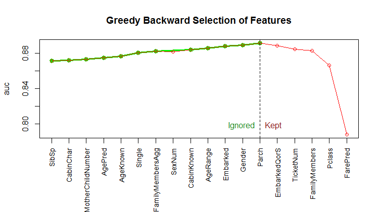
This subset of features has been obtained using a backwards version of the stepwise feature selection presented in our previous post (Random Forest, Forward Feature Selection & Grid Search). Bear in mind that those features have been selected using a random forest algorithm, which vastly differs from the method presented here. There might therefore be alternative ways of selecting a subset of features that would yield a better outcome… The result of the backwards stepwise algorithm is depicted in the following graph.
Autoencoder (Diabolo Network): Unsupervised Learning
We take advantage of the entire data set. In order to find adequately performing autoencoders, we rely on a grid search.
hyperParamsAutoencoder = list(
  hidden = list(c(11, 4, 11), c(10, 4, 10), c(9, 5, 9), c(9, 4, 9),
                c(7, 4, 7), c(8, 5, 8), c(8, 4, 8), c(8, 3, 8), c(7, 3, 7)),
  activation = c("Tanh")
)

h2o.rm("grid_autoencoder")
gridAutoencoder <- h2o.grid(
  x = predictors,
  autoencoder = TRUE,
  training_frame = trainUnsupervised,
  hyper_params = hyperParamsAutoencoder,
  search_criteria = list(strategy = "Cartesian"),
  algorithm = "deeplearning",
  grid_id = "grid_autoencoder",
  reproducible = TRUE,
  seed = 1,
  variable_importances = TRUE,
  categorical_encoding = "AUTO",
  score_interval = 10,
  epochs = 800,
  adaptive_rate = TRUE,
  standardize = TRUE,
  ignore_const_cols = FALSE)
The following table summarizes the grid results (it is sorted increasingly by ‘mse’):
  activation      hidden                   mse
1       Tanh   [9, 5, 9] 0.0026951381426859795
2       Tanh [10, 4, 10] 0.0028120481438311516
3       Tanh [11, 4, 11]  0.003175176064226341
4       Tanh   [7, 4, 7]  0.003811161604814563
5       Tanh   [9, 4, 9]  0.004018492030187388
6       Tanh   [8, 4, 8]  0.004980247622738063
...
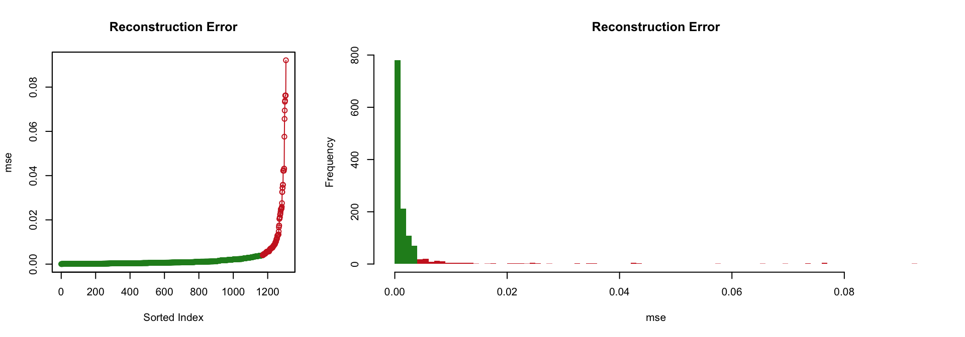
Considering the “best” autoencoder (i.e., the one with the lowest ‘mse’, which is the one with the hidden layers [9, 5, 9]), the two following figures illustrate the fact that it performs rather well; only a limited portion of the input signal could not be reconstructed.
Pretrained Neural Networks: Supervised Learning
Now we use the labaled data set (train) to turn the autoencoders generated above into classifiers.
getDlClassifier <- function (autoencoder, predictors, response, trainSupervised) {

  dlSupervisedModel <- h2o.deeplearning(
    y = response, x = predictors,
    training_frame = trainSupervised,
    pretrained_autoencoder = autoencoder@model_id,
    reproducible = TRUE,
    balance_classes = TRUE,
    ignore_const_cols = FALSE,
    seed = 1,
    hidden = autoencoder@parameters$hidden,
    categorical_encoding = "AUTO",
    epochs = autoencoder@parameters$epochs,
    standardize = TRUE,
    activation = autoencoder@parameters$activation)

  return (dlSupervisedModel)
}
Results
Here is the head of the sorted grid result—decreasingly by validAcc (accuracy achieved on the validation set); then, increasingly by pre-train ‘mse’. The column index is just a way for us to retrieve the prediction associated with the row.
> print(head(dfResults), row.names = FALSE)
  validAcc Threshold HiddenLayers PretrainMse index
 0.8913043       0.6    (9, 5, 9) 0.002695138     1
 0.8913043       0.5    (7, 4, 7) 0.003811162     4
 0.8913043       0.4    (9, 4, 9) 0.004018492     5
 0.8913043       0.5    (8, 5, 8) 0.010625935     8
 0.8695652       0.5  (10, 4, 10) 0.002812048     2
 0.8695652       0.5  (11, 4, 11) 0.003175176     3
Submitting the first row’s model (index 1) yielded the accuracy of 0.80383 on Kaggle. ■
License and Source Code
© 2017 Loic Merckel, Apache v2 licensed. The source code is available on both Kaggle and GitHub.
-
We recently posted a solution, Random Forest, Forward Feature Selection & Grid Search ↩