Kaggle's Mercedes Problem: PCA & Boosting
In an attempt to tackle the Kaggle’s Mercedes problem, we present a preliminary approach for dimensionality reduction reposing on principal component analysis. We first train a gradient boosting machine (GBM) using the entire set of features (baseline); then we attempt to improve the baseline result by reducing the feature dimensionality (a doing motivated by the fact that the number of features is large compared to the number of rows).
It turned out that our attempt was in vain; we found that using principal components as features did not yield a good outcome.
The feature tinkering part might be overly shallow, we probably need to further the initial preparation of features before moving on with training machines (as we say, garbage in, garbage out…).
Furthermore, we have only limited computational resources (a MacBook), and therefore, an extensive grid search was not really realistic. It is thus plausible that our result could be improved (to a certain extent) simply with more parameters tuning.
Features Tinkering
There are 378 features and only 4209 rows in the training set. We might be interested in reducing the number of features.
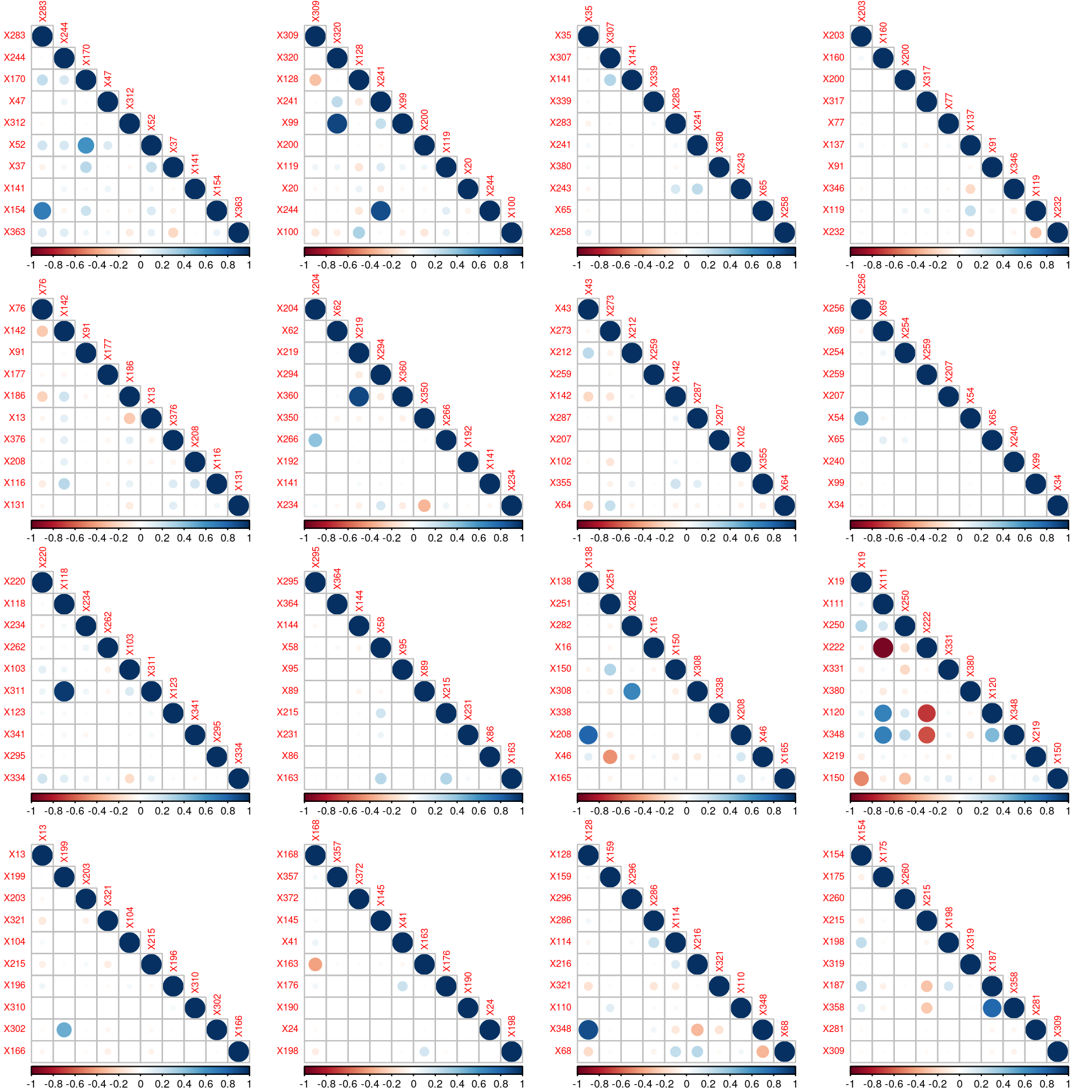
Since the features have been anonymized, it is it rather unclear what those features are. A rapid analysis reveals no missing values; besides, many columns appear to be quasi-constant.
There are 8 categorical variables, and 356 numerical variables with non-null standard deviation (those numerical values are either zero or one). The following graph reveals some correlation between the numerical features.
Convert Categorical Variables to Numerical
We use one-hot encoding.
##   X0 : 53 dummy varibles created
##   X1 : 27 dummy varibles created
##   X2 : 50 dummy varibles created
##   X3 : 7 dummy varibles created
##   X4 : 4 dummy varibles created
##   X5 : 33 dummy varibles created
##   X6 : 12 dummy varibles created
##   X8 : 25 dummy varibles created
Remove Constant Columns
The features X0ae, X0ag, X0an, X0av, X0bb, X0p, X2ab, X2ad, X2aj, X2ax, X2u, X2w, X5a, X5b, X5t, X5z, X11, X93, X107, X233, X235, X268, X289, X290, X293, X297, X330, X347 are constant in the training set, and thus dropped.
Remove Outlier from Response
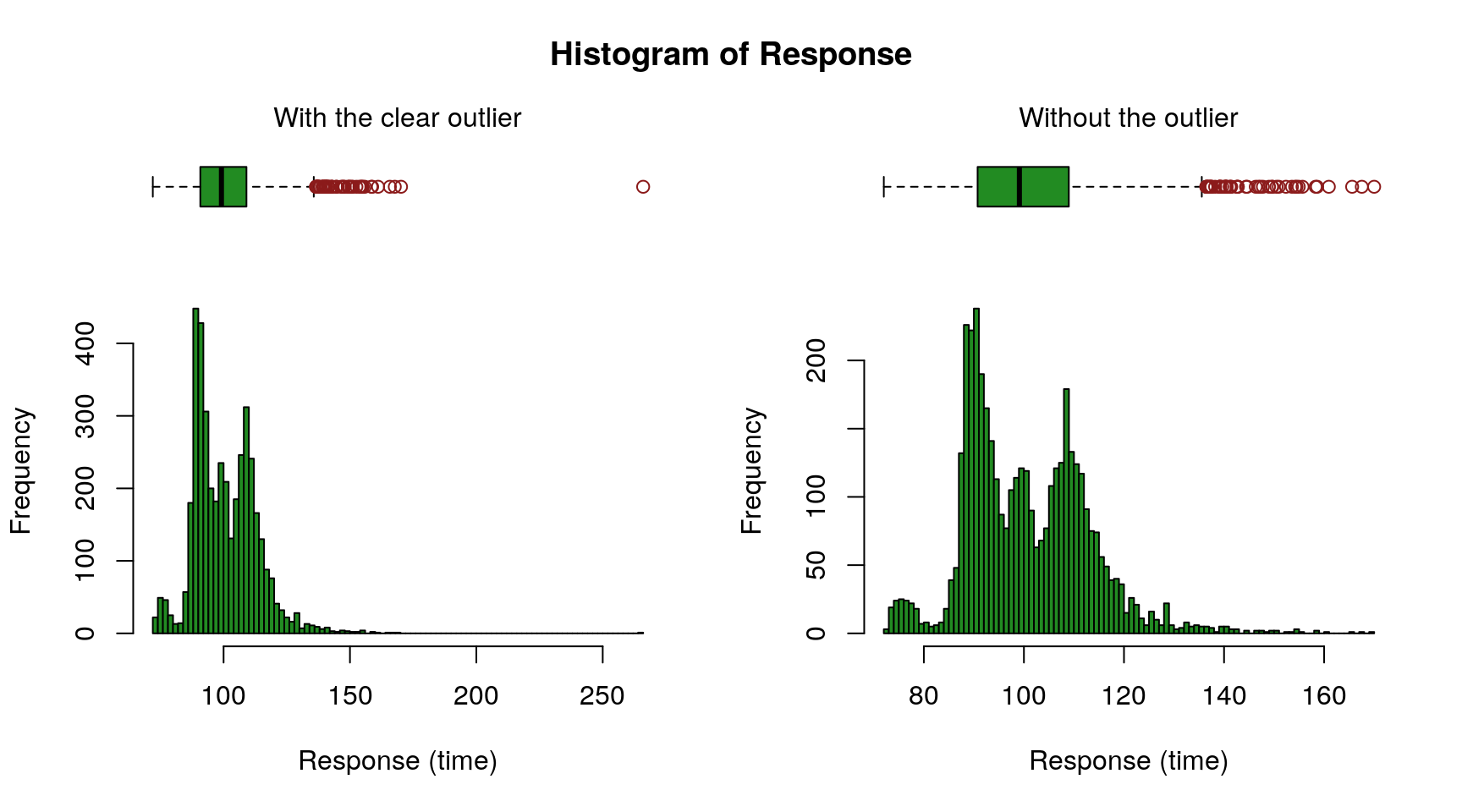
The figure above (left) reveals a clear outlier with a response time above 250. Let’s remove that likely spurious row.
numX <- numX[-which(numX$y > 250), ]
The right chart shows the resulting distribution.
Examine Possible Duplicated Rows
duplicatedRows <- duplicated(numX[, setdiff(names(numX), c("y", "ID"))])
There are 298 rows with identical features (except for the ID and the response).
formula <- getFormula (
  response = "y",
  features = setdiff(names(numX), c("y", "ID")),
  factorResponse = FALSE)

index <- 1
duplicatedRowResponse <- list()
aggNumX <- aggregate(formula, data = numX, drop = TRUE,
                     FUN = function (ys) {
                       if (length(ys) > 1) {
                         duplicatedRowResponse[[paste0(index)]] <- ys
                         duplicatedRowResponse <<- duplicatedRowResponse
                         index <<- index + 1
                       }
                       return(mean(ys))
                     })
It is interesting to observe that with the exact same configuration the testing times differ (and quite significantly for certain configurations—as depicted by the figure below). This is perhaps due to imperfection of the measuring device or perhaps human factors (tests not fully automated).
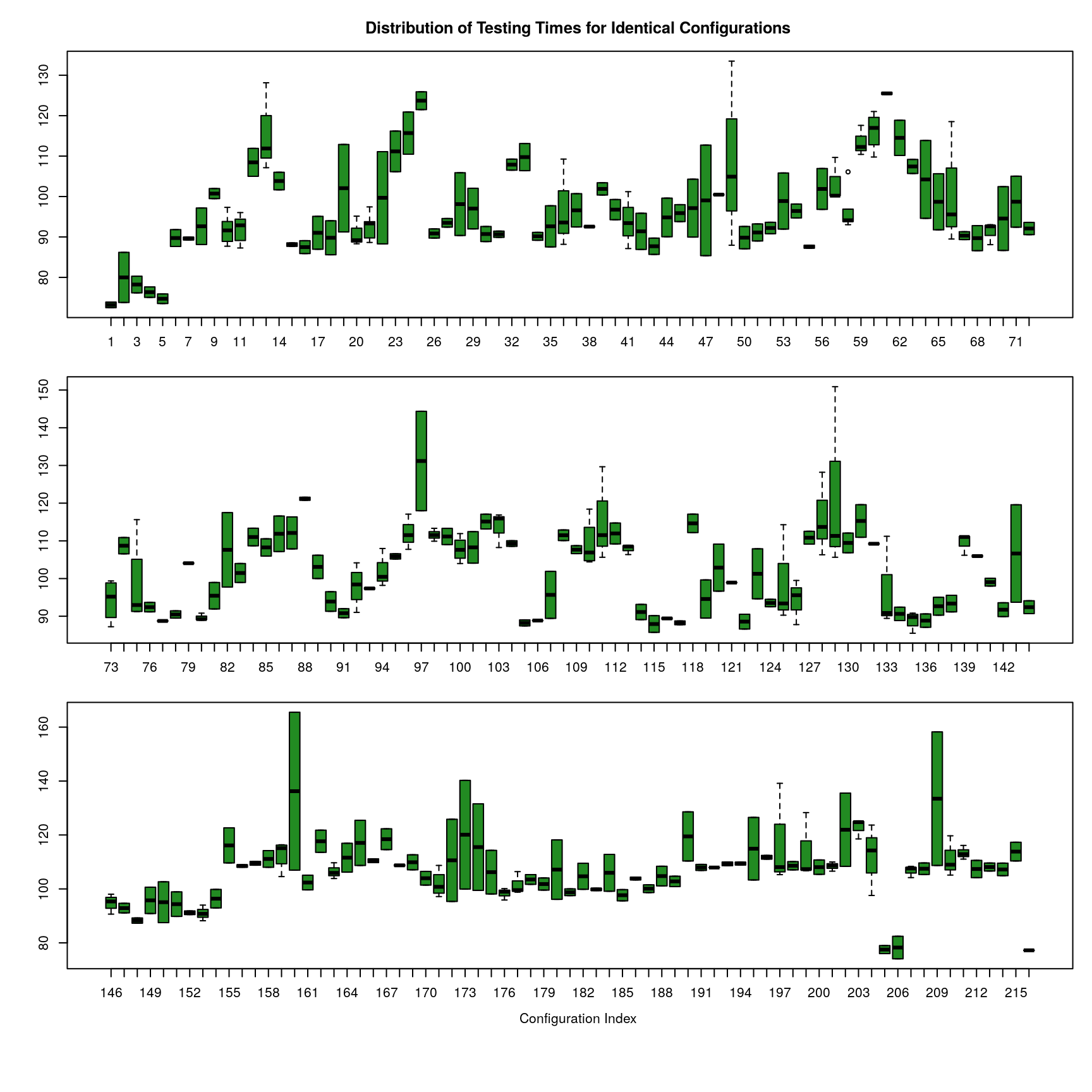
The problem for our regression model is that such discrepancies might confuse the machine… (especially the number of rows is not that large…)
Let’s aggregate those duplicated rows by identical features and set the response to the mean of their responses. Doing so, the already small number of rows further diminishes, but we might still gain from it.
One can remark that the IDs are lost, but we do not need them on the training set. Let’s add a dummy column ID so that all data sets are consistent.
numX <- cbind(ID = 0, aggNumX)
Baseline (Gradient Boosting Machine without Feature Reduction)
We try using the entire set of features.
The two following vectors of indexes to ignore should be identical given that ID is consistently the first column and response the last one.
indexToIgnoreTrain <- c(grep(paste0("^", response, "$"), names(train)),
                   grep("^ID$", names(train)))

indexToIgnoreTest <- c(grep(paste0("^", response, "$"), names(test)),
                        grep("^ID$", names(test)))
Note that we rely on XGBoost for the GBM training, in concert with the caret package for both grid search and cross-validation. Due to severe limitations in computational resources, the grid only spans very narrow ranges for hyper-parameters (consequently, we might very well miss more adequate settings). The situation is even worse on Kaggle (a 3-folds cross-validation with a two-row grid reaches the time out; hence the only one row grid below—it is still useful for when the script is executed on a decent machine, it is easy to expend the grid).
xgbGrid <- expand.grid(
  nrounds = c(400),
  eta = c(0.01),
  max_depth = c(4),
  gamma = 0,
  colsample_bytree = c(0.8),
  min_child_weight = c(3),
  subsample = c(0.7))

xgbTrControl <- trainControl(
  method = "cv",
  number = 3,
  verboseIter = FALSE,
  returnResamp = "final",
  allowParallel = TRUE)

set.seed(1)
xgbBaseline <- train(
  x = data.matrix(train[, -indexToIgnoreTrain]),
  y = train[[response]],
  trControl = xgbTrControl,
  tuneGrid = xgbGrid,
  method = "xgbTree",
  metric = "Rsquared",
  nthread = parallel:::detectCores())
Summary of the training:
## eXtreme Gradient Boosting
##
## 3910 samples
##  551 predictor
##
## No pre-processing
## Resampling: Cross-Validated (3 fold)
## Summary of sample sizes: 2607, 2607, 2606
## Resampling results:
##
##   RMSE      Rsquared
##   8.012706  0.6024303
##
## Tuning parameter 'nrounds' was held constant at a value of 400
##  0.8
## Tuning parameter 'min_child_weight' was held constant at a value of
##  3
## Tuning parameter 'subsample' was held constant at a value of 0.7
A more extensive grid search could lead to improved performance, but we are quite limited in computational resources…
We can submit to Kaggle’s LB to see how well the baseline model performs on the test set.
resultBaseline <- predict(xgbBaseline, data.matrix(test[, -indexToIgnoreTest]))
saveResult(Xt$ID, resultBaseline, "result-baseline")
Dimensionality Reduction
Principal Component Analysis (PCA)
We can include the test set into the PCA, but we must bear in mind that it is definitely not a good practice (to say it euphemistically), for the test set becomes part of the training process (basically, the resulting model might perform well on this test set, but might miserably fail to generalize to a new unseen data set). Here we do it because we won’t have any new data…
pcaTrain <- rbind(
  train[, predictors],
  test[, predictors])
pC <- prcomp(pcaTrain, center = normalize, scale. = normalize)
stdDev <- pC$sdev
propotionOfVarianceExplained <- stdDev^2 /sum(stdDev^2)
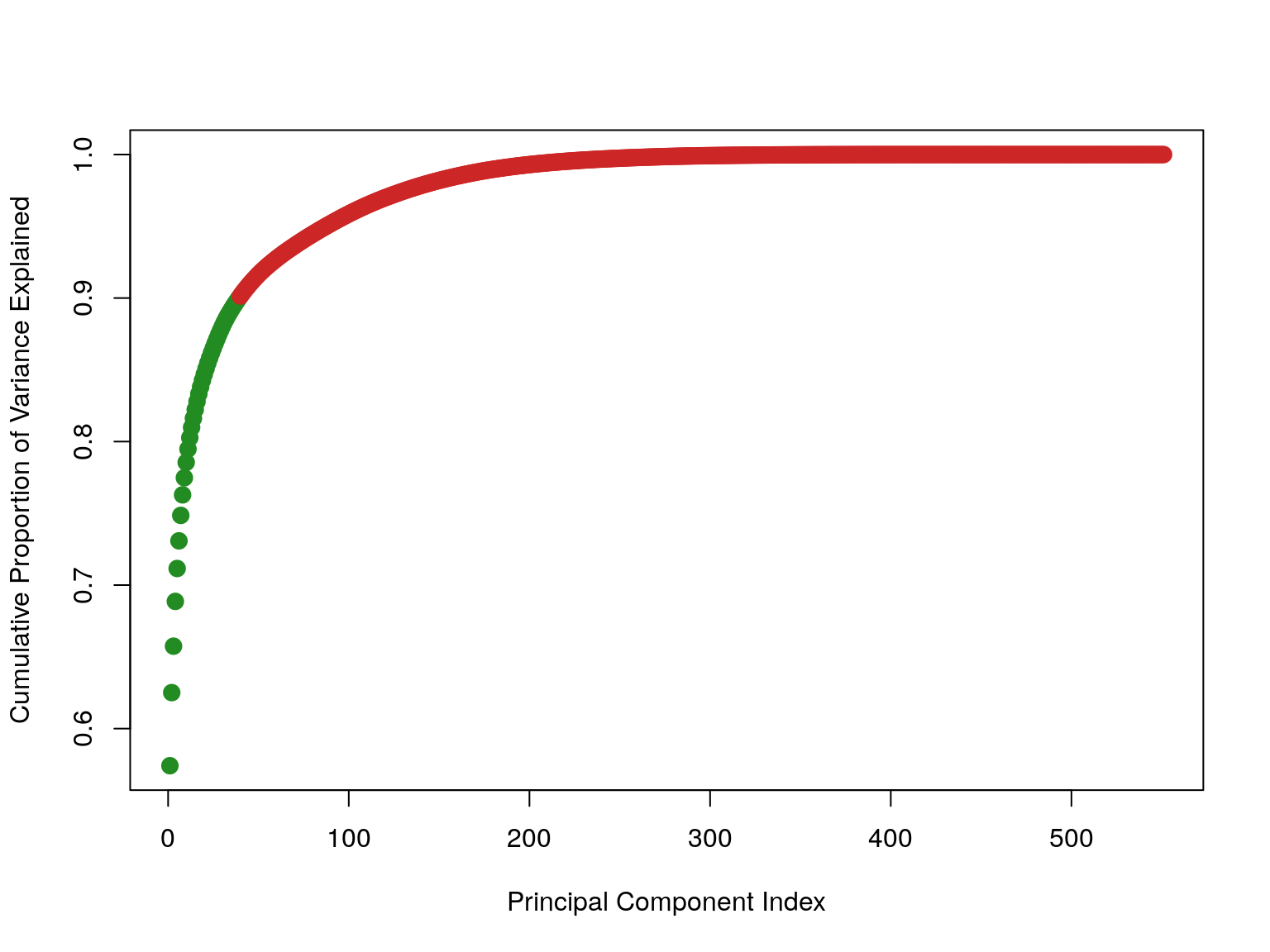
The first 40 explained 90% of the variance in the data.
Gradient Boosting Machine
trainReduced <- as.data.frame(predict(pC, newdata = train[, predictors]))
testReduced <- as.data.frame(predict(pC, newdata = test[, predictors]))
We select the 40 first components.
trainReduced <- trainReduced[, 1:numberOfComponents]
testReduced <- testReduced[, 1:numberOfComponents]
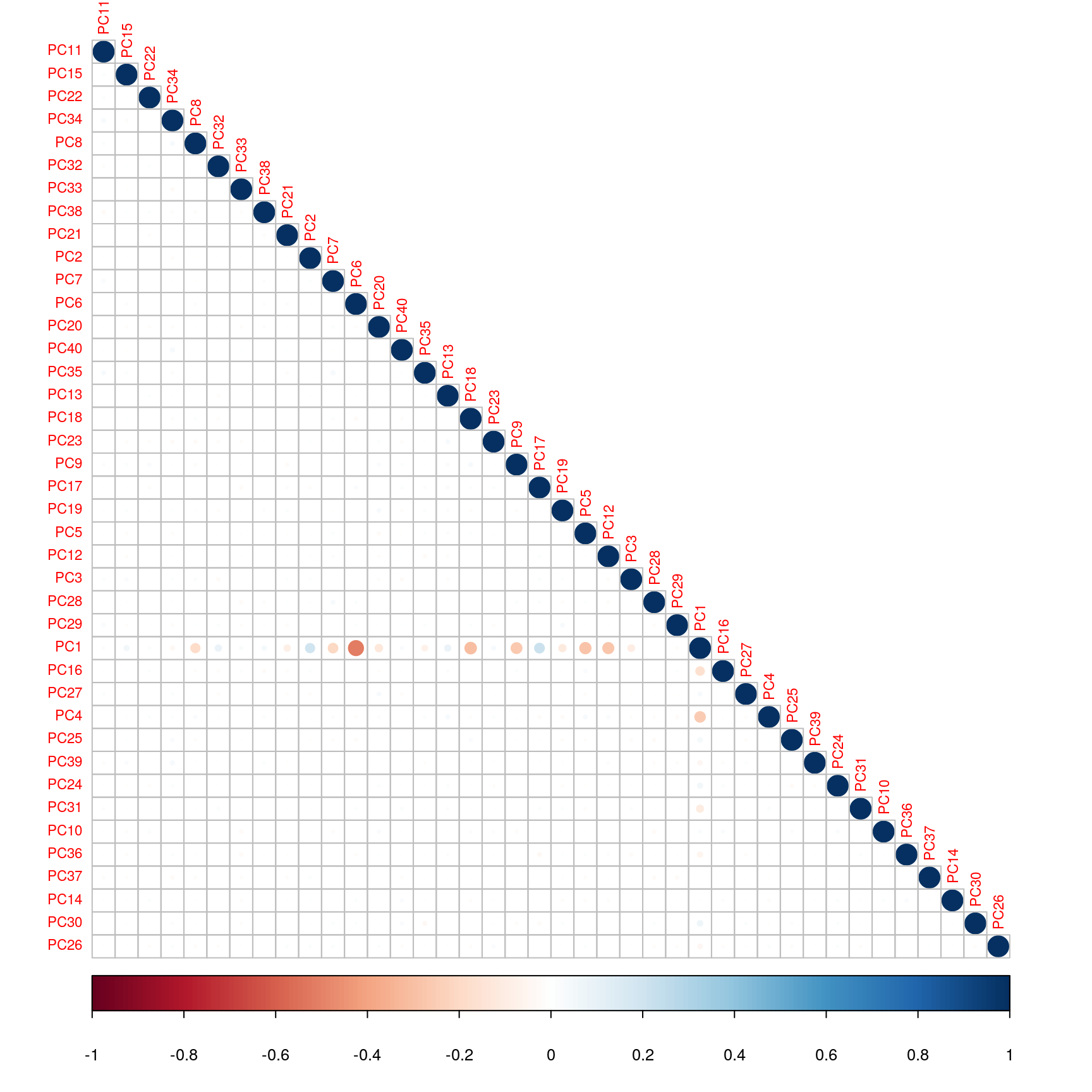
We can verify visually that there is only very few correlations between those components.
Add the column to predict.
trainReduced[[response]] <- train[[response]]
testReduced[[response]] <- NA
We train the GBM.
xgbGrid <- expand.grid(
  nrounds = c(400),
  eta = c(0.01),
  max_depth = c(6, 8),
  gamma = 0,
  colsample_bytree = c(0.8),
  min_child_weight = c(3),
  subsample = c(0.7))

xgbPca <- train(
  x = data.matrix(trainReduced[, -indexToIgnoreTrain]),
  y = trainReduced[[response]],
  trControl = xgbTrControl,
  tuneGrid = xgbGrid,
  method = "xgbTree",
  metric = "Rsquared",
  nthread = parallel:::detectCores())
Summary of the training:
## eXtreme Gradient Boosting
##
## 3910 samples
##   40 predictor
##
## No pre-processing
## Resampling: Cross-Validated (3 fold)
## Summary of sample sizes: 2607, 2607, 2606
## Resampling results across tuning parameters:
##
##   max_depth  RMSE      Rsquared
##   6          8.616416  0.5391570
##   8          8.655893  0.5350727
##
## Tuning parameter 'nrounds' was held constant at a value of 400
##  0.8
## Tuning parameter 'min_child_weight' was held constant at a value of
##  3
## Tuning parameter 'subsample' was held constant at a value of 0.7
## Rsquared was used to select the optimal model using  the largest value.
## The final values used for the model were nrounds = 400, max_depth = 6,
##  eta = 0.01, gamma = 0, colsample_bytree = 0.8, min_child_weight = 3
##  and subsample = 0.7.
Oops! Quite disenchanting outcome…
Predict the testing time on the test set—although, judging from the reported performance, it might not be necessary to submit anything out of that model to the Kaggle’s LB… The baseline result should be less embarrassing… (We got 0.55383 with a variant of the baseline case.)
resultPca <- predict(xgbPca, data.matrix(testReduced[, -indexToIgnoreTest]))
saveResult(Xt$ID, resultPca, "result-pca")
Concluding Remarks
It is a bit disappointing to observe no improvement after reducing the number of features using PCA; and even worse, we get some noticeable degradation of the baseline result. Sometimes things like that happen… A more thorough feature tinkering might help here to reduce the number of features and achieve better performance! ■
License and Source Code
© 2017 Loic Merckel, Apache v2 licensed. The source code is available on both Kaggle and GitHub.