Predicting Web Traffic: HoltWinters & ARIMA

Note: this post is a replication of our kernel published on Kaggle—Preliminary Investigation: HoltWinters & ARIMA.

Here we present a very simplistic, to the point of being rather naive, approach to the Kaggle’s Web Traffic Time Series Forecasting problem. Some aspects of dealing with time series in R are from A Little Book of R For Time Series (Coghlan, 2015). Each row (i.e., page) is considered individually, which might fail to capture correlations and other interactions between pages.

Forecasting Web Traffic for the Entire Data Set

setnames(keys, "Page", "PageWithDate")
n <- nchar("_0000-00-00")
keys[, Page := substr(PageWithDate, 0, nchar(PageWithDate) - n)]
keys[, Date := substr(PageWithDate, nchar(PageWithDate) - n + 2, nchar(PageWithDate))]
rm (n)

# 1: ARIMA or 2: HoltWinters
kMethod <- 2
kH <- 31 + 28 + 1 # from Jan 1, 2017 to Mar 1, 2017
kUseTsClean <- TRUE
kSmoothOrder <- 0 # no smoothing if <= 0

i <- 1
forecastWebTraffic <- function(x) {
  row <- unname(unlist(x))

  predictions <- tryCatch({
    if (kUseTsClean) {
      rowTs <- tsclean(ts(row, frequency = 365.25, start = c(2015, 7, 1)))
    } else {
        # outliers (Hampel's test)
        minMaxThreshold <- 3 * c(-1, 1) * 1.48 * mad(row, na.rm = TRUE) 
                            + median(row, na.rm = TRUE)  
        row[row < minMaxThreshold[1]] <- NA 
        row[row > minMaxThreshold[2]] <- NA 
        
        # missing values
        rowTs <- ts(row, frequency = 365.25, start = c(2015, 7, 1))
        if (anyNA(rowTs)) {
          rowTs <- na.interpolation(rowTs, option = "spline")
        }
    }
    if (kSmoothOrder > 0) {
      smoothed <- ma(rowTs, order = kSmoothOrder)
      indexes <- (kSmoothOrder %/% 2 + 1):(length(rowTs) - (kSmoothOrder %/% 2 + 1))
      rowTs[indexes] <- smoothed[indexes]
      rm(smoothed, indexes)
    }
    
    # predictions
    if (kMethod == 1) {
      fit <- auto.arima(rowTs)
    } else {
      fit <- HoltWinters(rowTs, beta = FALSE, gamma = FALSE)
    }
    predictions <- forecast(fit, h = kH, fan = FALSE)
  }, error = function(e) {
    predictions <- data.frame(mean = rep(0, kH))
  })
  
  i <<- i + 1
  if (kIsOnKaggle && i == 100) {
    stop("Stop execution to prevent time out on Kaggle", call. = FALSE)
  }
  
  return (as.list (as.numeric(predictions$mean)))
}

vars <- names(X[, -1])
try(X[, 
      c(unique(keys$Date)) := forecastWebTraffic (.SD), 
      .SDcols = vars, by = 1:nrow(X)])

meltX <- melt(
  X[, which(names(X) %in% c(unique(keys$Date), "Page")), with = FALSE], 
  measure.vars = unique(keys$Date), 
  variable.name = "Date", 
  value.name = "Visits")
meltX$Date <- as.character(meltX$Date)

mergeKeysMeltX <- merge(keys, meltX, by=c("Page", "Date"), all.x = TRUE)

fwrite(
  mergeKeysMeltX[, c("Id", "Visits")], 
  file = file.path(
           ".", 
           paste0(
             "output-", 
             ifelse(kMethod == 1, "arima", "holtwinters"), 
             ".csv"), 
           fsep = .Platform$file.sep), 
  row.names = FALSE,  quote = FALSE)

One can find further details about the Hampel’s test for outlier detection in Scrub data with scale-invariant nonlinear digital filters.

HoltWinters Illustration with a Single Page

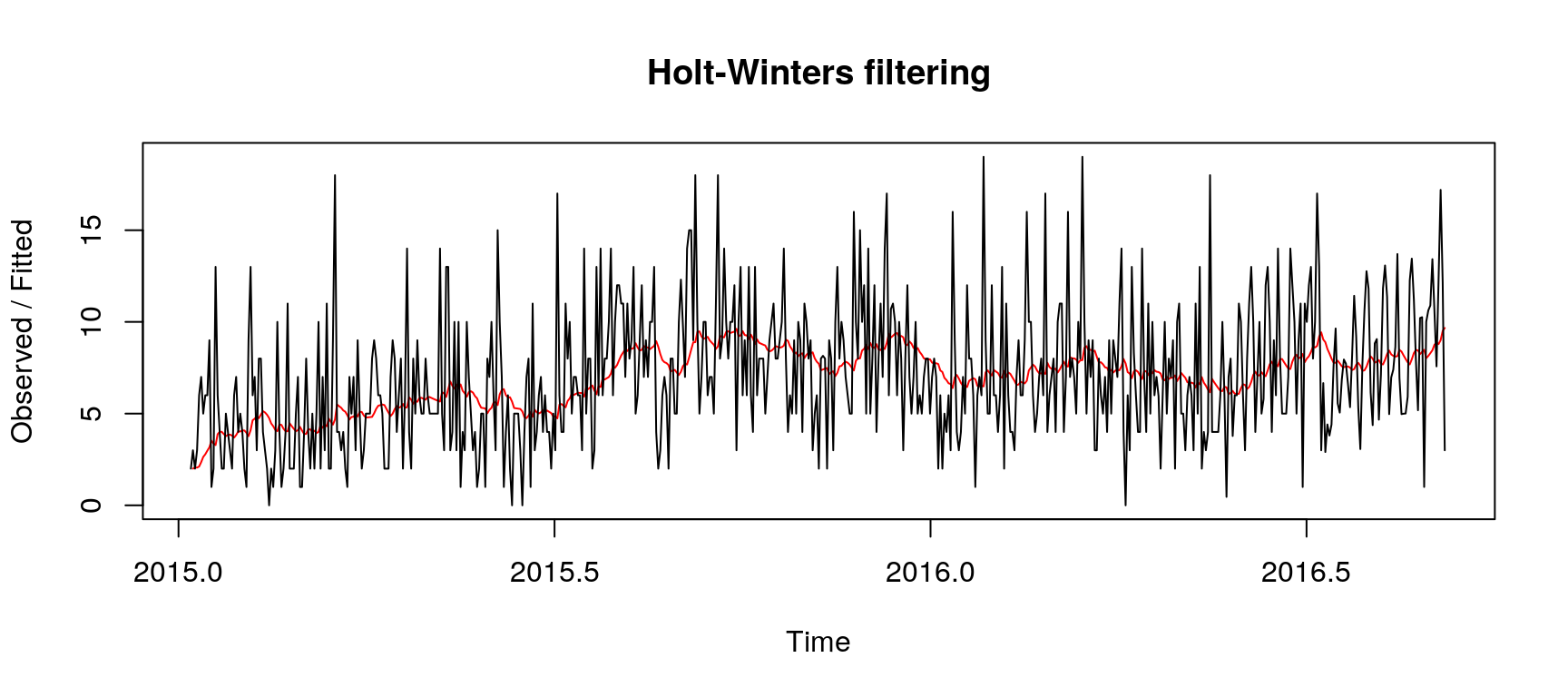
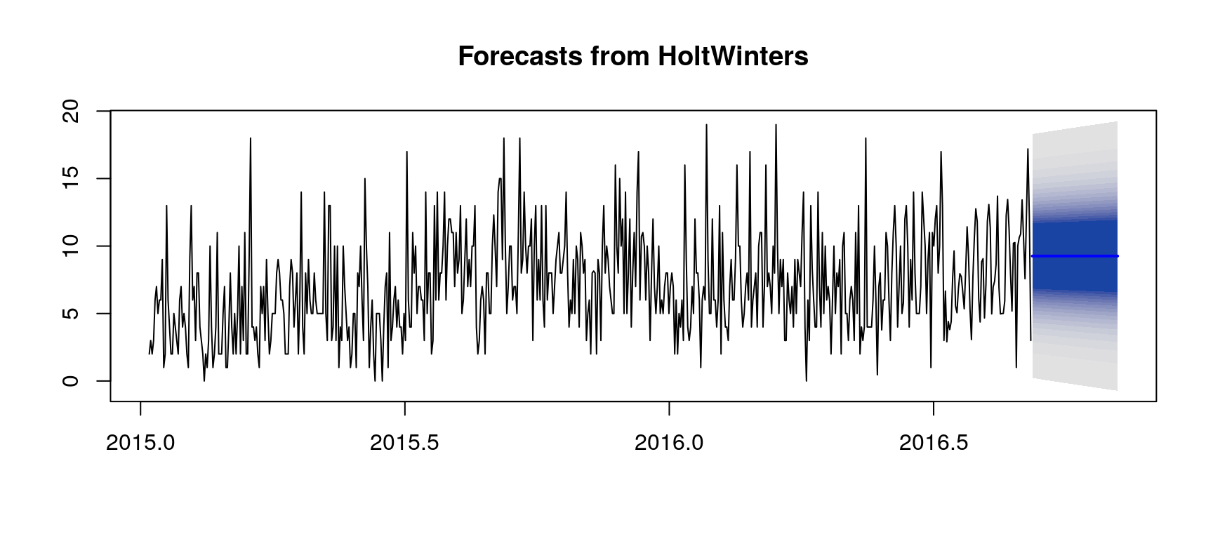
Here we consider the page 大月薰_zh.wikipedia.org_all-access_spider.

row <- unname(unlist(X[rowIndex, -1, with = FALSE]))
rowTs <- removeOutliersAndImputNa (row)
fit <- HoltWinters(rowTs, beta = FALSE, gamma = FALSE)
predictions <- forecast(fit, h = kH, fan = TRUE)

ARIMA Illustration with a Single Page

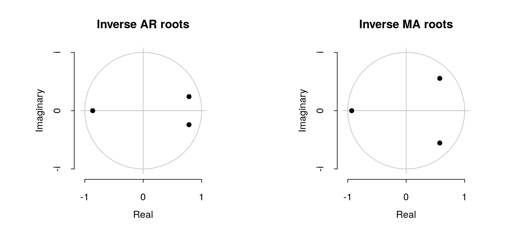
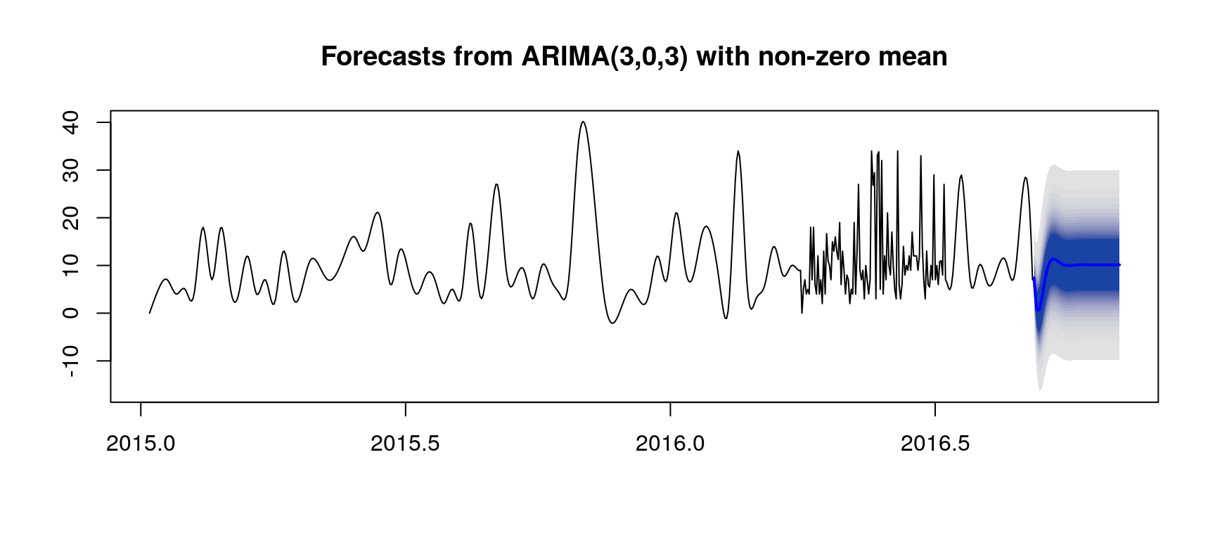
Here we consider the page Missing9_zh.wikipedia.org_all-access_spider.

row <- unname(unlist(X[rowIndex, -1, with = FALSE]))
rowTs <- removeOutliersAndImputNa (row)
fit <- auto.arima(rowTs)
predictions <- forecast(fit, h = kH, fan = TRUE)

License and Source Code

References

Coghlan, A. (2015). A Little Book of R for Time Series. https://goo.gl/toSpsH