Autoencoder and Deep Features
In this tutorial-like kernel, using data from New York City Taxi Trip Duration, we use the autoencoder and deeplearning capability of the H2O framework to explore deep features. Such an approach provides a means of reducing features (Hinton & Salakhutdinov, 2006)—although here there is no need, for the number of features is already small. It also offers a way to leverage unlabelled data—a technique called semi-supervised learning. The kernel Diabolo Trick: Pre-train, Train and Solve gives a concrete example. Finally, it is perhaps worth noting that deep features are the backbone of some transfer learning techniques.
Features Tinkering
First, we remove the column dropoff_datetime, as otherwise there is no point to predict the duration of the trip… We could just precisely calculate it…
X[, dropoff_datetime := NULL]
Outliers
Pickup Location
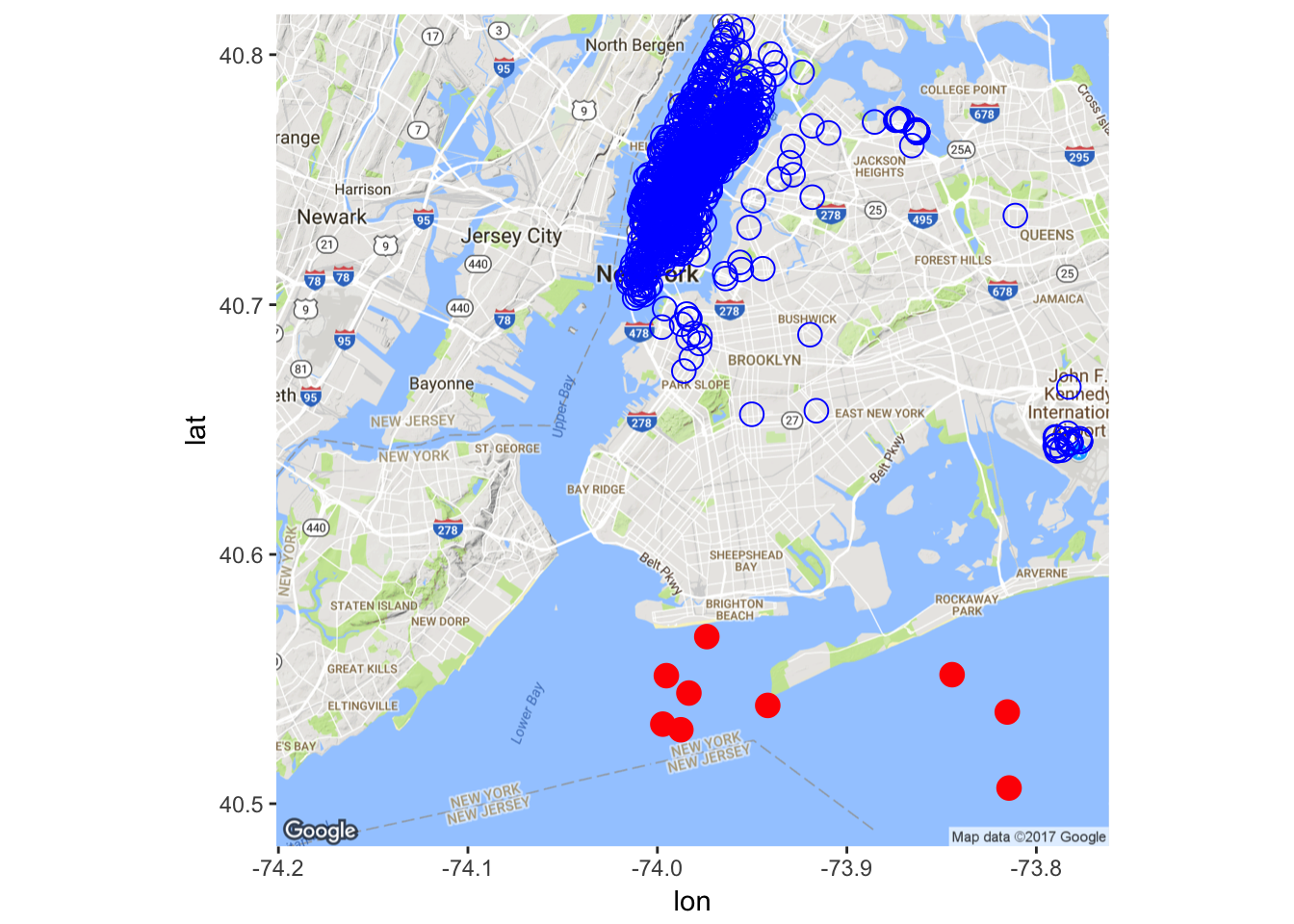
There seems to be some outliers in the dataset. Let’s remove some of them (obviously, a better way should be devised here, for the current naive implementation misses some outliers while removing some non-outliers).
X <- X[-which(X$pickup_longitude > -74
             & X$pickup_latitude < 40.57), ]
Trip Duration
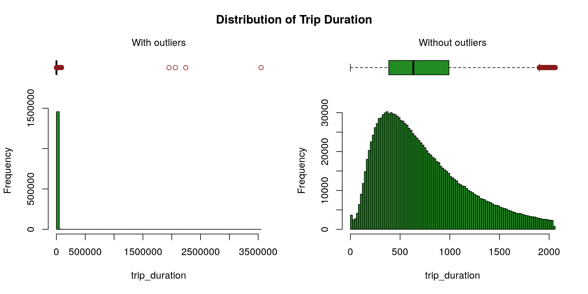
We rely on the Hampel’s test to compute the maximum threshold above which values are declared spurious. One can find further details about the Hampel’s test for outlier detection in Scrub data with scale-invariant nonlinear digital filters.
X <- X[-which(X$trip_duration > maxThreshold), ]
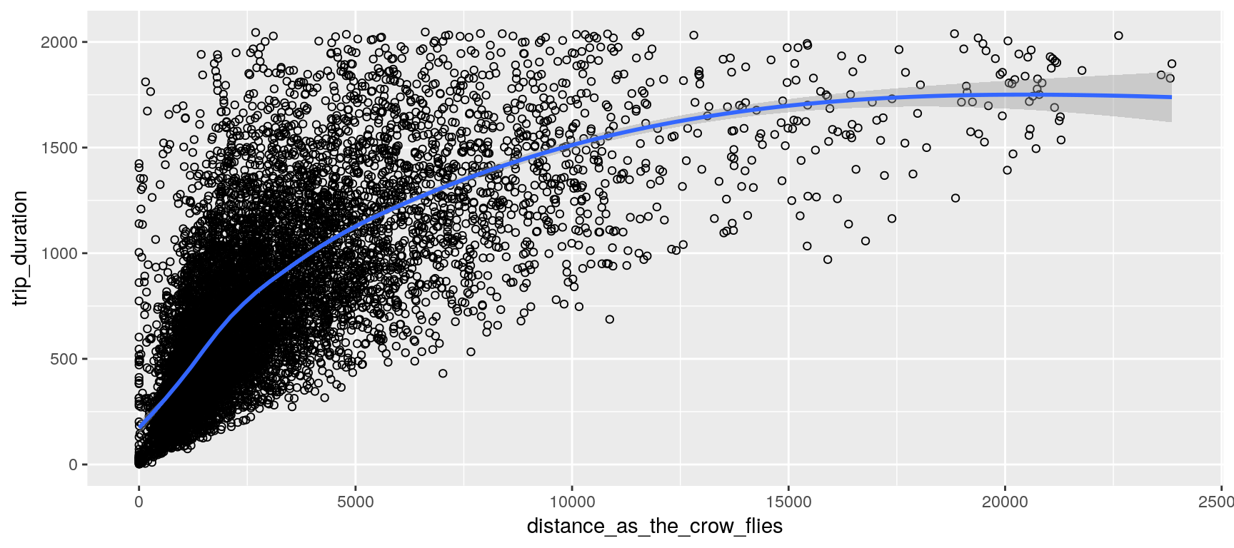
Locations and Distances
We assume that the earth’s surface forms a perfect sphere; so that we can conveniently use the haversine formula to estimate each trip distance as the crow flies. (This distance should constitute a rough estimation of the covered distance; at least it gives a minimum.)
X[, distance_as_the_crow_flies := distHaversine(
    data.table(pickup_longitude, pickup_latitude),
    data.table(dropoff_longitude, dropoff_latitude))]

Xt[, distance_as_the_crow_flies := distHaversine(
    data.table(pickup_longitude, pickup_latitude),
    data.table(dropoff_longitude, dropoff_latitude))]
Pickup Date
We add the two new features wday and hour.
X[, pickup_datetime := fastPOSIXct (pickup_datetime, tz = "EST")]
X[, wday := wday(pickup_datetime)]
X[, hour := hour (pickup_datetime)]

Xt[, pickup_datetime := fastPOSIXct (pickup_datetime, tz = "EST")]
Xt[, wday := wday(pickup_datetime)]
Xt[, hour := hour (pickup_datetime)]
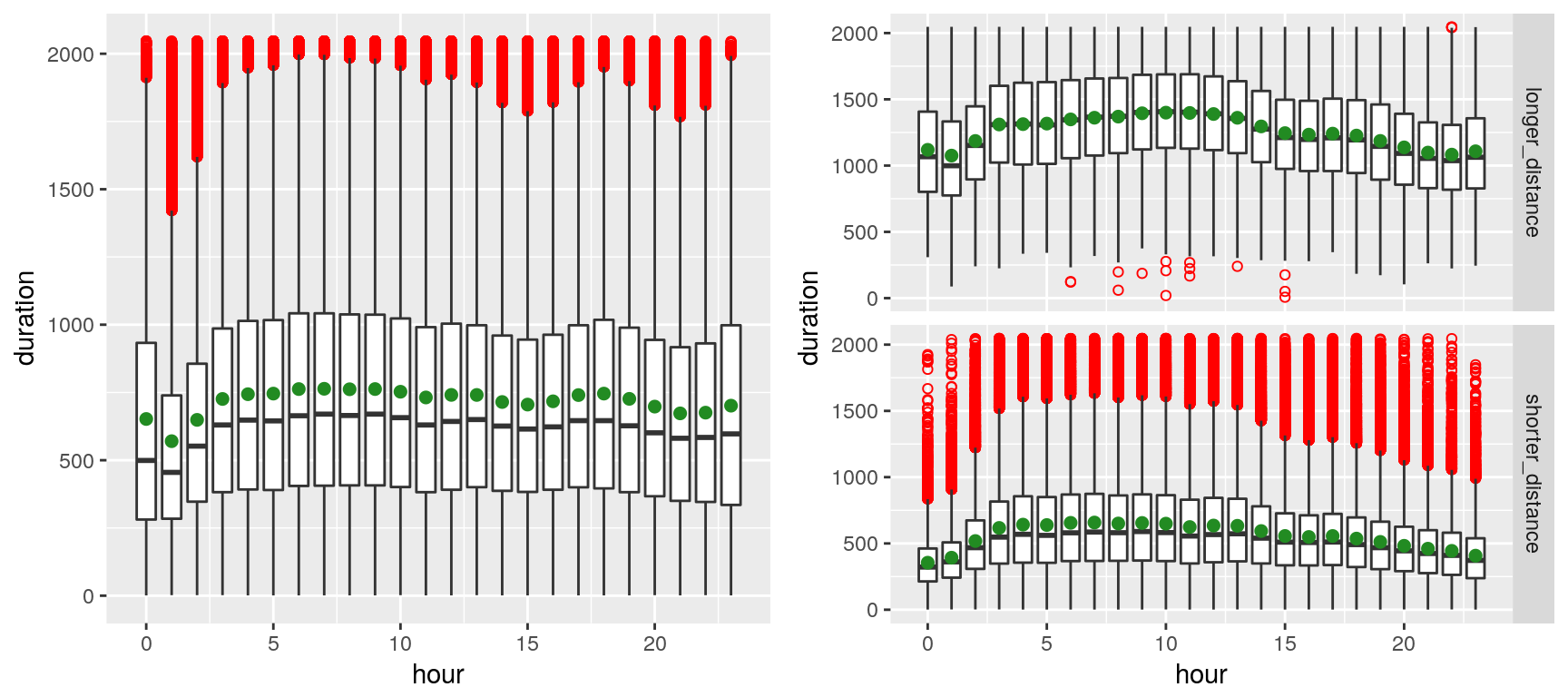
We can observe, on the left plot, the presence of outliers (red dots)—which markedly shift the mean (green spot) from the median—presumably due to the volatility of the traffic in New York. The right plot contrasts shorted distances (arbitrarily chosen as less than 4 Km) with longer distances. Outliers appear to merely plague the shorter distances (which is fairly intuitive, especially given that many of the shorter-distance trips appear to be within Manhattan).
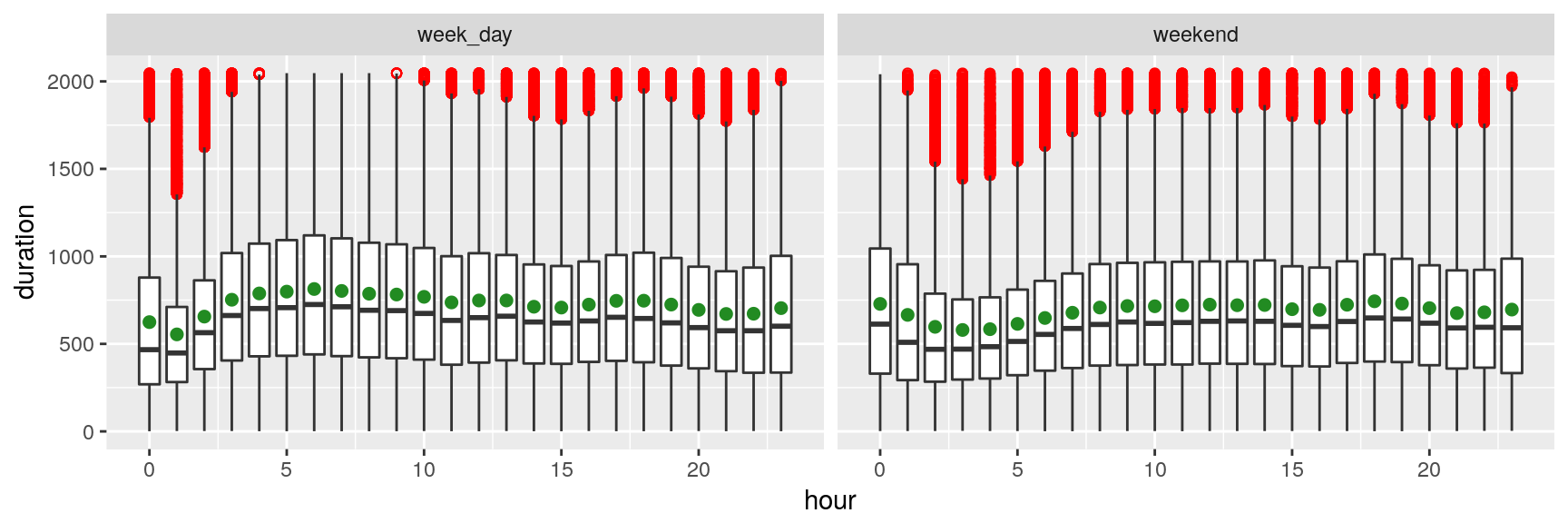
The plot above suggests that trip durations are longer late at night during the weekend, whereas they tend to be longer early morning (4~8) during the weekdays (depicting the rush hours of commuters). That sounds rather unsurprising…
Convert Categorical Variables to Numerical
There is 1 categorical variables, and there are 9 numerical variables with non-null standard deviation.
X[, store_and_fwd_flag := ifelse (store_and_fwd_flag == "N", 0, 1)]
Deep Features
Convert to H2O Frames
if (kIsOnKaggle) {
  # we reduce the training set size to avoid time out
  set.seed(1)
  trainIndexes <- createDataPartition(
    y = X[["trip_duration"]], p = 0.1, list = FALSE)
  X <- X[trainIndexes, ]
  rm(trainIndexes)
}
train <- as.h2o(X)
predictors <- setdiff (names(X), c(toIgnore))
Autoencoder (Diabolo Network)
if (kIsOnKaggle) {
  hyperParamsAutoencoder = list(
    hidden = list(c(8, 4, 8), c(8, 3, 8), c(7, 3, 7), c(6, 3, 6)),
    activation = c("Tanh"))
} else {
  hyperParamsAutoencoder = list(
    hidden = list(c(11, 8, 11), c(10, 8, 10), c(9, 5, 9), c(8, 5, 8),
                  c(7, 5, 7), c(6, 5, 6), c(11, 7, 11), c(10, 7, 10),
                  c(9, 4, 9), c(8, 4, 8), c(7, 4, 7), c(6, 4, 6),
                  c(11, 6, 11), c(10, 6, 10), c(9, 3, 9), c(8, 3, 8),
                  c(7, 3, 7), c(6, 3, 6), c(11, 5, 11), c(10, 5, 10),
                  c(11, 4, 11), c(10, 4, 10), c(11, 8, 5, 8, 11)),
    activation = c("Tanh"))
}

gridAutoencoder <- h2o.grid(
  x = predictors,
  autoencoder = TRUE,
  training_frame = train,
  hyper_params = hyperParamsAutoencoder,
  search_criteria = list(strategy = "Cartesian"),
  algorithm = "deeplearning",
  grid_id = "grid_autoencoder",
  reproducible = TRUE,
  seed = 1,
  variable_importances = TRUE,
  categorical_encoding = "AUTO",
  score_interval = 10,
  epochs = 800,
  adaptive_rate = TRUE,
  standardize = TRUE,
  ignore_const_cols = FALSE)
The following table summarizes the grid results (it is sorted increasingly by ‘mse’):
| activation | hidden | mse | |
|---|---|---|---|
| 1 | Tanh | [8, 4, 8] | 2.2115573249558083E-5 |
| 2 | Tanh | [8, 3, 8] | 6.43305860410787E-4 |
| 3 | Tanh | [7, 3, 7] | 6.519543824901826E-4 |
| 4 | Tanh | [6, 3, 6] | 6.730825397209355E-4 |
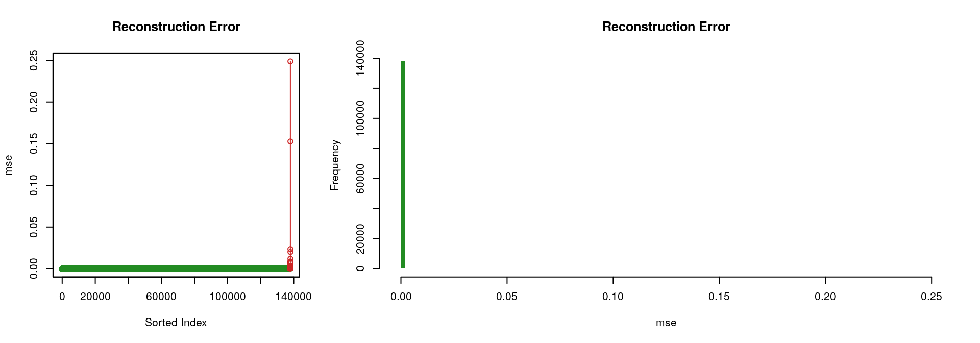
Considering the “best” autoencoder (i.e., the one with the lowest ‘mse’, which is the one with the hidden layers [8, 4, 8]), the two following figures illustrate the fact that it performs rather well; only a limited portion of the input signal could not be reconstructed.
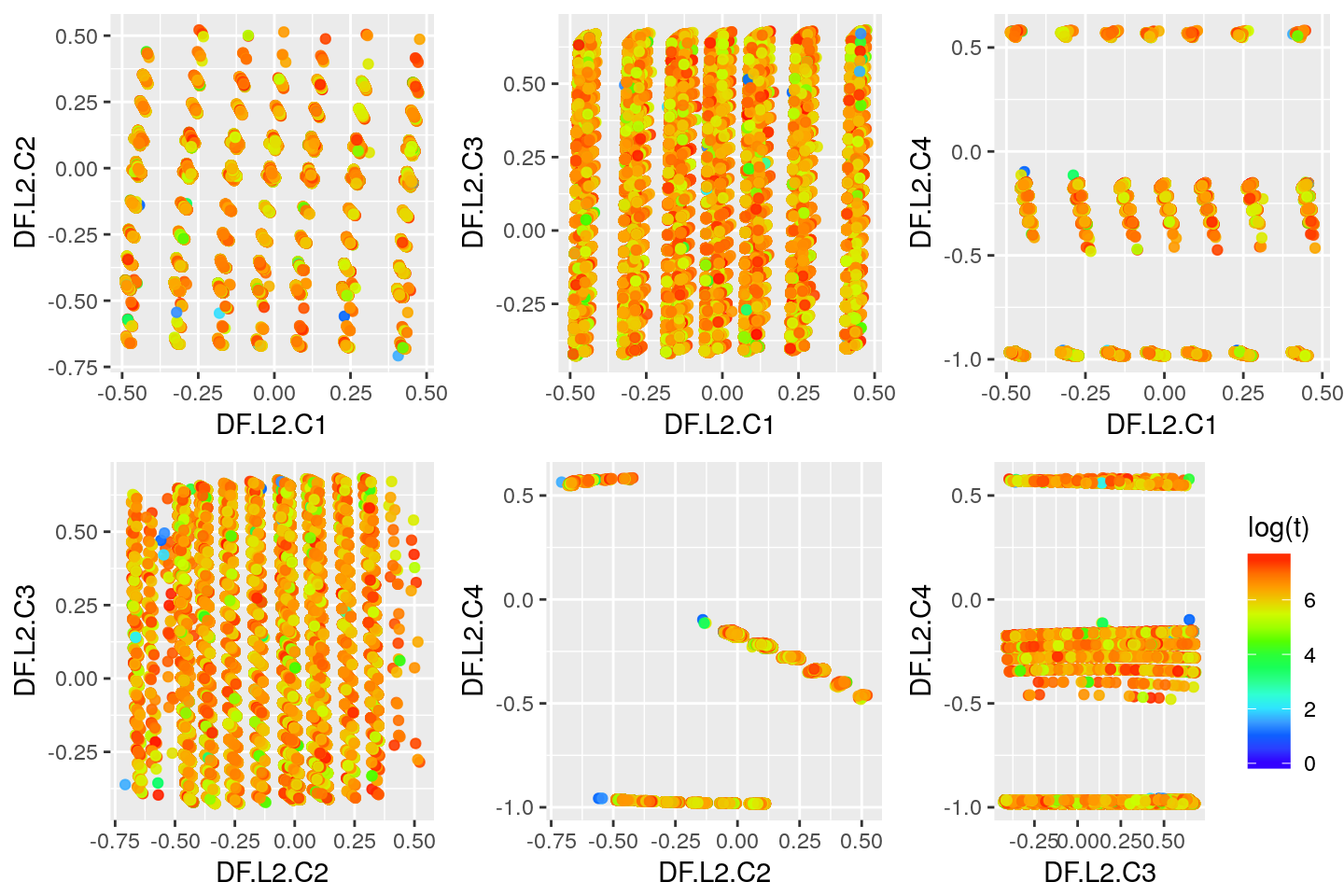
Deep Features Visualization
Second Layer
layer <- 2
deepFeature2 <- h2o.deepfeatures(bestAutoencoder, train, layer = layer)
data <- as.data.frame(deepFeature2)
data$log_trip_duration <- log(X$trip_duration)

summary(data)
##     DF.L2.C1           DF.L2.C2           DF.L2.C3          DF.L2.C4
##  Min.   :-0.48997   Min.   :-0.70796   Min.   :-0.4266   Min.   :-0.9829
##  1st Qu.:-0.28532   1st Qu.:-0.45367   1st Qu.:-0.1012   1st Qu.:-0.9661
##  Median :-0.05116   Median :-0.04050   Median : 0.1981   Median :-0.9644
##  Mean   :-0.05273   Mean   :-0.18749   Mean   : 0.1545   Mean   :-0.5969
##  3rd Qu.: 0.12783   3rd Qu.:-0.01238   3rd Qu.: 0.4004   3rd Qu.:-0.1662
##  Max.   : 0.47711   Max.   : 0.52161   Max.   : 0.6832   Max.   : 0.5846
##  log_trip_duration
##  Min.   :0.000
##  1st Qu.:5.951
##  Median :6.446
##  Mean   :6.376
##  3rd Qu.:6.894
##  Max.   :7.624
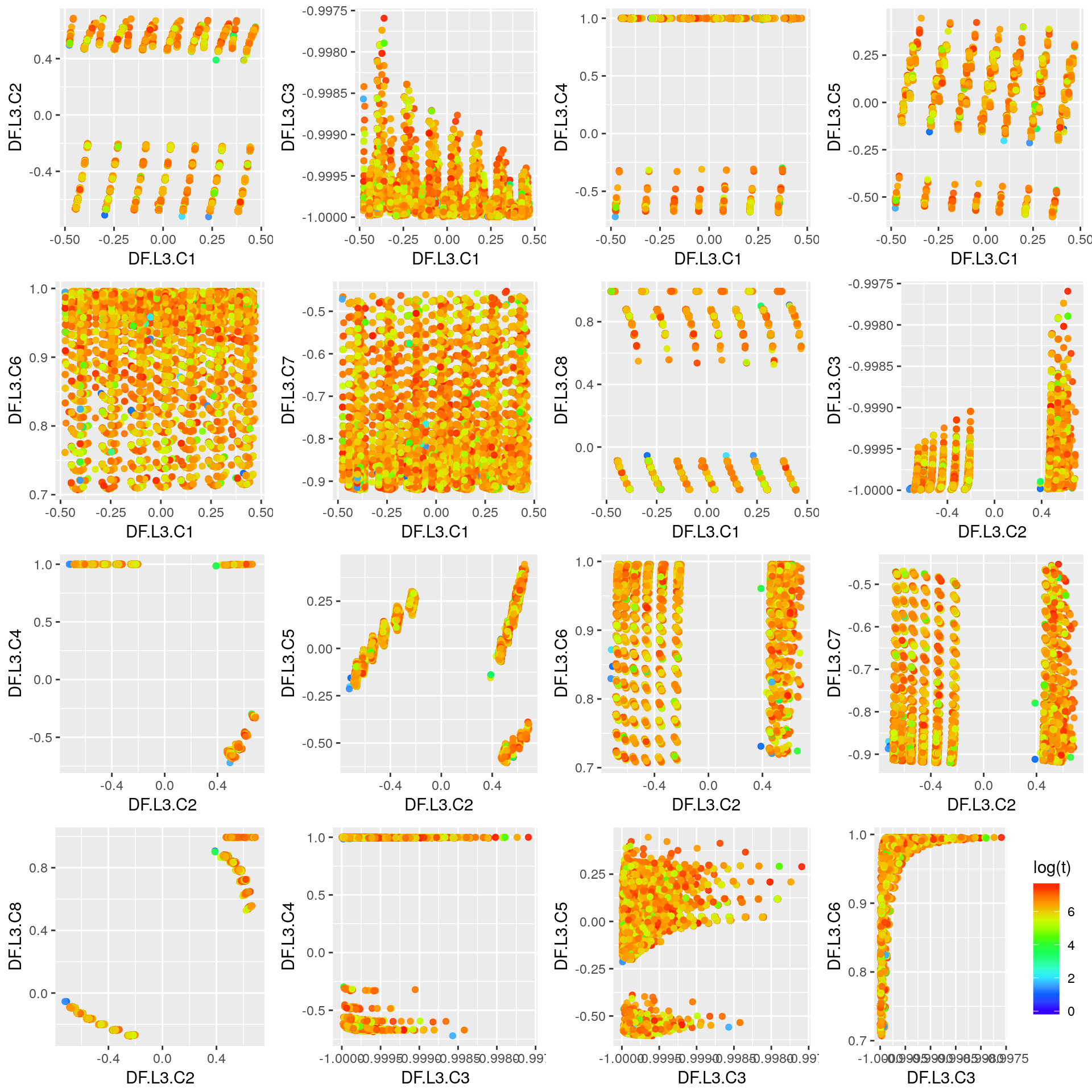
Third Layer
layer <- 3
deepFeature3 <- h2o.deepfeatures(bestAutoencoder, train, layer = layer)
data <- as.data.frame(deepFeature3)
data$log_trip_duration <- log(X$trip_duration)

summary(data)
##     DF.L3.C1           DF.L3.C2           DF.L3.C3          DF.L3.C4
##  Min.   :-0.47818   Min.   :-0.72271   Min.   :-1.0000   Min.   :-0.7213
##  1st Qu.:-0.14682   1st Qu.:-0.66474   1st Qu.:-1.0000   1st Qu.: 0.9941
##  Median : 0.02289   Median :-0.32626   Median :-0.9999   Median : 0.9997
##  Mean   : 0.03259   Mean   :-0.09229   Mean   :-0.9998   Mean   : 0.9889
##  3rd Qu.: 0.26142   3rd Qu.: 0.46748   3rd Qu.:-0.9998   3rd Qu.: 0.9997
##  Max.   : 0.47005   Max.   : 0.68681   Max.   :-0.9976   Max.   : 1.0000
##     DF.L3.C5           DF.L3.C6         DF.L3.C7          DF.L3.C8
##  Min.   :-0.60460   Min.   :0.7071   Min.   :-0.9202   Min.   :-0.27290
##  1st Qu.:-0.12264   1st Qu.:0.8905   1st Qu.:-0.8631   1st Qu.:-0.09507
##  Median :-0.03823   Median :0.9506   Median :-0.8037   Median :-0.09062
##  Mean   :-0.03506   Mean   :0.9294   Mean   :-0.7637   Mean   : 0.33366
##  3rd Qu.: 0.01698   3rd Qu.:0.9848   3rd Qu.:-0.6714   3rd Qu.: 0.87194
##  Max.   : 0.44521   Max.   :0.9960   Max.   :-0.4528   Max.   : 0.99467
##  log_trip_duration
##  Min.   :0.000
##  1st Qu.:5.951
##  Median :6.446
##  Mean   :6.376
##  3rd Qu.:6.894
##  Max.   :7.624
Predictions Using Deep Features and GBM
We use the second layer of the autocencoder (bestAutoencoder) and the gradient boosting machine algorithm offered by H2O (h2o.gbm). Those are arbitrary choices for the purpose of exemplifying a use of deep features.
layer <- 2
Get Deep Features & Split Data
deepFeatureTrain <- h2o.deepfeatures(bestAutoencoder, train, layer = layer)
deepFeatureTrain[["trip_duration"]] <- as.h2o(X$trip_duration)
splits <- h2o.splitFrame(
  data = deepFeatureTrain,
  ratios = c(0.7),
  seed = 1
)
trainDf <- splits[[1]]
validDf <- splits[[2]]
Grid Search
deepfeatures <- setdiff(names(deepFeatureTrain), c("trip_duration"))

if (kIsOnKaggle) {
  hyperParamsGbm <- list(
    max_depth = c(3, 4),
    min_split_improvement = c(0, 1e-6))
} else {
  hyperParamsGbm <- list(
    max_depth = seq(3, 15, 2),
    sample_rate = seq(0.2, 1, 0.01),
    col_sample_rate_per_tree = seq(0.2, 1, 0.01),
    col_sample_rate_change_per_level = seq(0.6, 1.4, 0.02),
    min_rows = 2^seq(0, log2(nrow(train))-3, 1),
    nbins = 2^seq(2, 10, 1),
    nbins_cats = 2^seq(1, 4, 1),
    histogram_type = c("UniformAdaptive", "QuantilesGlobal", "RoundRobin"),
    min_split_improvement = c(0, 1e-8, 1e-6, 1e-4))
}

gridGbm <- h2o.grid(
  hyper_params = hyperParamsGbm,
  search_criteria = list(strategy = "Cartesian"),
  algorithm = "gbm",
  grid_id = "grid_gbm",
  x = deepfeatures,
  y = "trip_duration",
  training_frame = trainDf,
  validation_frame = validDf,
  nfolds = 0,
  ntrees = ifelse(kIsOnKaggle, 200, 1000),
  learn_rate = 0.05,
  learn_rate_annealing = 0.99,
  max_runtime_secs = ifelse(kIsOnKaggle, 120, 3600),
  stopping_rounds = 5,
  stopping_tolerance = 1e-5,
  stopping_metric = "MSE",
  score_tree_interval = 10,
  seed = 1,
  fold_assignment = "AUTO",
  keep_cross_validation_predictions = FALSE)

sortedGridGbm <- h2o.getGrid("grid_gbm", sort_by = "mse", decreasing = TRUE)
| max_depth | min_split_improvement | mse | |
|---|---|---|---|
| 1 | 3 | 1.0E-6 | 187782.15952044743 |
| 2 | 3 | 0.0 | 187782.15952044743 |
| 3 | 4 | 0.0 | 183708.52366487522 |
| 4 | 4 | 1.0E-6 | 183708.52366487522 |
Best Model & Performance on the Validation Set
bestGbmModel <- h2o.getModel(sortedGridGbm@model_ids[[1]])
perf <- h2o.performance(bestGbmModel, newdata = validDf)
## H2ORegressionMetrics: gbm
##
## MSE:  187782.2
## RMSE:  433.3384
## MAE:  349.3986
## RMSLE:  0.7301732
## Mean Residual Deviance :  187782.2
Retrain the Best Model Using the Entire Train Set
Here we use k-folds cross validation to evaluate the final model (trained using the entire train set—i.e., rbind(trainDf, validDf)).
nfolds <- ifelse(kIsOnKaggle, 2, 8)
finalModel <- do.call(h2o.gbm,
                      {
                        p <- bestGbmModel@parameters
                        p$model_id = NULL
                        p$training_frame = h2o.rbind(trainDf, validDf)
                        p$validation_frame = NULL
                        p$nfolds = nfolds
                        p
                      })
finalModel@model$cross_validation_metrics_summary
## Cross-Validation Metrics Summary:
##                               mean           sd  cv_1_valid  cv_2_valid
## mae                       350.8387   0.10633527   350.68832    350.9891
## mean_residual_deviance   189029.88    113.88638   188868.83   189190.94
## mse                      189029.88    113.88638   188868.83   189190.94
## r2                     0.029764593 1.9335767E-4 0.030038042 0.029491143
## residual_deviance        189029.88    113.88638   188868.83   189190.94
## rmse                     434.77563   0.13097145    434.5904   434.96085
## rmsle                   0.73611194 0.0039748037  0.73049074   0.7417332
Test Set & Submission
deepFeatureTest <- h2o.deepfeatures(bestAutoencoder, test, layer = layer)
deepFeatureTest[["trip_duration"]] <- as.h2o(Xt$trip_duration)

pred <- h2o.predict (finalModel, newdata = deepFeatureTest)

fwrite(data.table(id = Xt$id, trip_duration = as.vector(pred$predict)),
       file = file.path(".", paste0("output-gbm-", Sys.Date(), ".csv"),
                        fsep = .Platform$file.sep),
       row.names = FALSE,  quote = FALSE)
Remark
In general, using the top model out of the grid search might not be the wisest approach. Instead, considering the k best models might yield improved performances (k > 1). An easy way to use k models is to average their predicted probabilities. A more sophisticated way consists in using ensemble learning (super learner), for which the choice of the meta-learner can help to even further improve the result (e.g., see H2O’s documentation on Stacked Ensembles).
Predictions Using Pretrained Neural Networks
This section describes an alternative approach to the previous section and is presented in a dedicated kernel: Deep Semi-supervised Learning. ■
License and Source Code
© 2017 Loic Merckel, Apache v2 licensed. The source code is available on both Kaggle and GitHub.
References
- Hinton, G. E., & Salakhutdinov, R. R. (2006). Reducing the Dimensionality of Data with Neural Networks. Science, 313(5786), 504–507. https://goo.gl/6GjADx