Risklet

Risklet is a minimal (toy) webapp that implements a few typical risk measurement techniques for a common stock portfolio.

This page describes how the portfolio expected return (simple and logarithmic), volatility, Sharpe ratio, value at risk (and expected shortfall) and efficient frontier are calculated. Several of those aspects derive from modern portfolio theory (Markowitz, 1952; Markowitz, 1955), which reposes on unrealistic assumptions (Ledoit & Wolf, 2004; Elton & Gruber, 1997) among other problems (Michaud, 1989; Michaud, 2004). In practice, the estimation of the expected returns for the coming period remains challenging, for past returns seem not to be an indicator of future returns (Clarke et al., 2006). “Remember that all models are wrong; the practical question is how wrong do they have to be to not be useful” (Box & Draper, 1987, p. 74).

Besides the mathematical modeling, some technical points regarding the webapp itself (such as programming language and hosting) are briefly discussed.

Expected Return

Simple Return

Single Asset

Let \(C^{(a)} =\{c_0, \dots, c_N \}\) be the closing prices—assumed adjusted—of an asset \(a\) over \(N\) trading days—\(c_{N}\) being the latest observed price. The simple net return over the considered period is defined as \(sr^{(a)}_{0 \to N} = (c_N - c_0) \div c_0\). It represents the change in wealth over the period. It can be computed from daily returns by observing that \(1 + sr_{0 \to N}^{(a)}=\prod_{k=1}^{N} 1 + sr^{(a)}_k\), where \(sr_k^{(a)}=(c_k - c_{k-1}) \div c_{k-1}\), \(k \in [\![ 1 .. N ]\!]\), denotes the \(k\)-th daily return.

Assuming \(T\) trading days per year (e.g., for the US financial markets \(T=252\)), the \(N\) days can be expressed as \( N \div T \) year(s); the annualized return is then yielded by¹:

Portfolio

Let’s consider a portfolio \(P\) consisting of \(A\) constituents with returns \(\{sr^{(1)}, \dots, sr^{(A)}\}\) and respective weights \(\{\alpha_1, \dots, \alpha_A\}\) such that \(\sum_{i=1}^A \alpha_i = 1\). The expected yearly net simple return \(sr\) of \(P\) is given by

$$sr = \sum_{a = 1}^{A} \alpha_i \times sr^{(a)}. \tag{2}$$

Logarithmic Return

Single Asset

Using the same notation as above, the log net return over the considered period is defined as (Panna, 2017): \(lr_{0 \to N}^{(a)} = \ln \left( 1 + sr^{(a)}_{0 \to N} \right)\) \(= \ln(c_N \div c_0)\). From daily log returns: \(lr_{0 \to N}^{(a)} = \sum_{k=1}^{N} lr_{k}^{(a)}\), where \(lr_k^{(a)} = \ln(c_k \div c_{k-1})\), \(k \in [\![ 1 .. N ]\!]\), denotes the \(k\)-th daily log return.

Since the log return is time additive, the arithmetic average gives us the daily expected value, and the annualized log return is yielded by:

$$lr^{(a)} = \frac{T}{N}\sum_{k=1}^{N} lr_{k}^{(a)}. \tag{3}$$

Portfolio

Although log returns have the nice property of being time additive, the log return of \(P\) is not the weighted mean of its constituents’ log return. However, in many cases it provides a reasonable approximation (Panna, 2017, appx. A; Hudson & Gregoriou, 2015)

$$lr \approx \sum_{a = 1}^{A} \alpha_i \times lr^{(a)}. \tag{4}$$

This approximation can be justified using the Taylor series. Rozeff & Kinney (“Capital Market Seasonality: The Case of Stock Returns,” 1976) claims that in the context of stock returns \(\ln(1+r) \approx r\) is valid when \(r \leq 0.15\) (a claim not substantiated in the paper, but which implies that the quadratic terms and beyond—smaller than 0.01125 in absolute—are deemed negligible, as per the Taylor series), as highlighted by Hudson & Gregoriou: “it is important not to wrongly deduce from this that the mean of a set of returns measured using logarithmic returns is necessarily very similar to the mean of the same set of returns measured using simple returns” (“Calculating and Comparing Security Returns Is Harder than You Think: A Comparison between Logarithmic and Simple Returns,” 2015, p. 5). They established, by neglecting the cubic and higher terms in the Taylor series, “that the difference between mean log returns and mean simple returns depends on the variance of simple returns” (Hudson & Gregoriou, 2015, appx. A). It remains unclear to the author to which extent equation (6) provides a reasonable approximation (extremely volatile securities—showing a drastic change within a single day—are far from being uncommon on the market).

Note that \(lr\) can be precisely computed as \(\ln(\sum_{k=1}^{A} \alpha_k \times \exp(lr_k^{(a)}))\). However, in Risklet we have implemented equation (4).

Volatility

We now have our portfolio return (either an exact simple return or an approximation of its log return). From a risk assessment perspective, this only might appear as inadequate. A typical motivation to look at historical data for computing a parameter is the hope that it provides a reasonable estimation of its future value (forecast). However a single point estimate cannot possibly capture any of the uncertainty pertaining to that estimate². “An uncertain number is a shape known as its distribution” (Savage & Markowitz, 2009, chap. 8).

Measuring risk as the standard deviation, also referred to as volatility, is a common practice in finance (Baillie & DeGennaro, 1990) . Let \(r_k^{(a)}\), \((k, a) \in [\![ 1 .. N ]\!] \times [\![ 1 .. A ]\!]\) be the \(k\)-th daily return—either simple or logarithmic—of security \(a\). Under the assumptions that the daily returns are i.i.d. and additive, the yearly volatility \(\sigma\) is yielded by:

where \(i \in [\![ 1 .. A ]\!]\) and \((k, a) \in [\![ 1 .. N ]\!] \times [\![ 1 .. A ]\!]\). (Those matrix notations might not be conventional, but they should be quite explicit.)

There is one caveat regarding the simple returns, though. Simple returns are not additive but multiplicative. Given that the arithmetic mean is used for computing the daily expected return, and that the standard deviation measures the “spread” around that mean, using simple returns might render the interpretability of the result less meaningful.

However, Hudson & Gregoriou show that “the sample variance of log returns and the sample variance of simple returns are approximately equal” (“Calculating and Comparing Security Returns Is Harder than You Think: A Comparison between Logarithmic and Simple Returns,” 2015, appx. A). Their argumentation reposes on the Taylor series and neglects the cubic and higher terms. This result can easily be observed with Risklet when selecting and unselecting ‘Log return’.

Portfolio Efficient Frontier

Equations (2), (4) and (5) indicate that both the return, noted \(r\) (either simple or logarithmic) and the volatility \(\sigma\) of our portfolio \(P\) are function of the weights of each security \((\alpha_i)_{i \in [\![ 1 .. A ]\!]}\). The objective of a wise investor with a given risk appetite (i.e., \(\sigma\)) consists in getting the maximum possible return (i.e., \(r\)). Equivalently said, given a desired return, how one can minimize the risk of achieving it? Yet another, more formal, way to express it, is given a desired return \(r_d\) solve for \((\alpha_i)_{i \in [\![ 1 .. A ]\!]}\) the following constrained optimization:

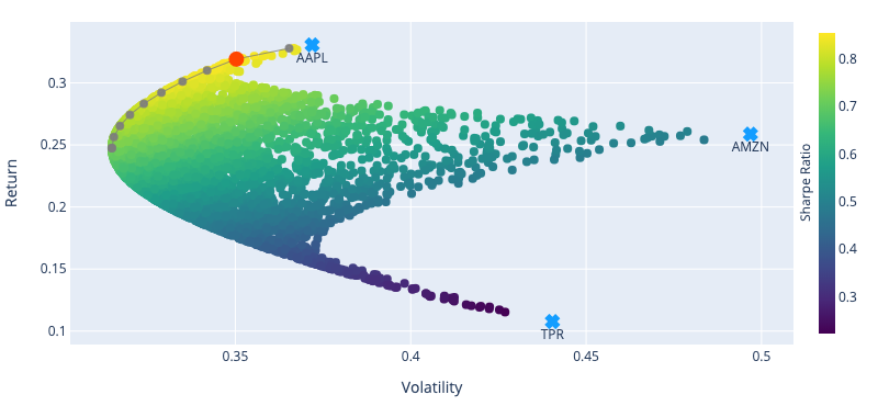
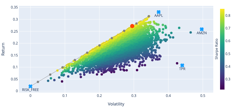
Markowitz (“Portfolio Selection,” 1952) has gained fame for addressing this problem, and was even awarded a Nobel prize. For a portfolio made exclusively of risky assets, the efficient frontier is a hyperbola (as depicted in fig. 1). However, when adding a risk-free asset, it becomes a line for which the y-intercept is the risk-free rate (as illustrated in fig. 2).

(Note that in the constraints of the optimization problem (6), \(r((\alpha_i)_{i \in [\![ 1 .. A ]\!]}) = r_d\) is sometimes specified as \(r((\alpha_i)_{i \in [\![ 1 .. A ]\!]}) \geq r_d\).)

Regarding the constraints, we can add \(\alpha_i \geq 0\), \(i \in [\![ 1 .. A ]\!]\) should short positions not be allowed.

Sharpe Ratio

The Sharpe ratio is a measure of performance rather than a measure of risk. Again noting \(r\) the portfolio return and \(\sigma\) its volatility, the Sharpe ratio is defined as

$$S = \frac{r - r_f}{\sigma}, \tag{7}$$

where \(r_f\) is the risk-free rate. It contrasts the excess return of the portfolio (over the risk-free rate) with the risk taken to achieve this excess. One can remark that \(S = S((\alpha_i)_{i \in [\![ 1 .. A ]\!]})\), and the optimal portfolio in terms of Sharpe ratio can be found by solving for \((\alpha_i)_{i \in [\![ 1 .. A ]\!]}\) the following constrained optimization: maximize \(S((\alpha_i)_{i \in [\![ 1 .. A ]\!]})\) subject to \(\sum_{i=1}^A \alpha_i = 1\).

There are other measures of performances such as the Sortino ratio (Sortino & Price, 1994) and the Treynor ratio (Hübner, 2005), and many more.

Value at Risk and Expected Shortfall

Value at risk (VaR) is a risk measure technique that focuses on potential losses (unlike volatility that gives an indication of the spread around the mean, i.e., potential losses as well as potential gains). VaR tells the maximum percentage—or amount—loss over a given time horizon with a specified confidence interval an investor can expect.

There are several methods to compute it, and each of those methods likely yields different figures. Risklet implements two of them: historical method and variance-covariance method. Currently the time horizon is fixed at one day.

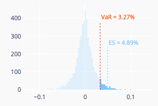
Let’s note \(\alpha\) the desired confidence interval. The historical method simply consists in taking the \(\alpha\)-th quantile of the historical loss distribution of the portfolio daily returns \(-\sum_{a = 1}^{A} \alpha_i \times r_{k}^{(a)}\), \(k \in [\![ 1 .. N ]\!]\). (Note the minus sign.) Here \(r_{k}^{(a)}\) can be either the simple daily return of the asset \(a\) or its approximate log return (see earlier discussion). The expected shortfall (ES) is the mean of the daily losses that are equal or greater than the VaR. Figure 3 (left) illustrates this method.

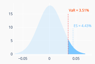
The variance-covariance method assumes that the portfolio return is normally distributed (perhaps, in practice, it may be a bit of a stretch an assumption, to say it mildly). The daily expected return \(r_d\) of the portfolio can be estimated by setting \(T=1\) in equation (1) for simple return and in equation (3) for log return. Likewise, the volatility \(\sigma_d\) can be obtained from equation (5). We have \(\text{VaR } = -r_d + z \times \sigma_d\), where \(z=\Phi^{-1}(\alpha)\), with \(\Phi^{-1}\) denoting the quantile function of the standard normal distribution. The expected shortfall is given by \(-r_d + \sigma_d \times \varphi(z) \div (1-\alpha) \), where \(\varphi\) is the normal probability density function. Figure 3 (right) illustrates this method.

Besides not being a coherent risk measure as it does not satisfy the sub-additivity property (by contrast, the expected shortfall is a coherent risk measure), a lot of criticisms seem to surround this measure. If one googles “value at risk criticism”, a plethora of relevant links will be suggested. One interesting reference is Against Value-at-Risk: Nassim Taleb Replies to Philippe Jorion.

Some Technical Aspects

This webapp is developed in Python (both the back end and the front end—using Dash Open Source). It currently runs on (hosted by) Google App Engine, which has the great advantage to offer a free quota. Cloud Firestore is used for caching data. A custom back end relying on Firestore for Flask-Caching has been implemented. This may sound a bit peculiar, for one might point out a typical use case for Flask-Caching (more generally caching) is to (i) alleviate the database storage load and (ii) provide a faster mechanism for retrieving the data. The reason for using Firestore lies in the fact that Firestore comes with a free quota, whereas the Google Memorystore for Redis does not.

The server is located in the US and the App Engine configuration is set to keep the resources consumption within the free quota. Consequently, the app may appear quite slow to many users. Bear in mind that this app is computationally intensive in the first place, and even with a cache mechanism (as already implemented) and a strong dedicated server located nearby, systematic real-time response would still be challenging to achieve.

In order to prevent excessive resource utilization, the current version limits the number of assets to 10 and the number of random portfolios generation (i.e. “number of simulations”) to 1000.

Acknowledgement

The ‘New York Oil and Gas’ dashboard from the Dash App Gallery has been used for building this webapp. The source code is available on GitHub.

The data are fetched from either Alpha Vantage or from Yahoo! finance (via the yfinance library).

References

1. Baillie, R. T., & DeGennaro, R. P. (1990). Stock returns and volatility. Journal of Financial and Quantitative Analysis, 203–214.
2. Box, G. E. P., & Draper, N. R. (1987). Empirical model-building and response surfaces. New York ; Chichester : Wiley.
3. Clarke, R. G., De Silva, H., & Thorley, S. (2006). Minimum-variance portfolios in the US equity market. The Journal of Portfolio Management, 33(1), 10–24.
4. Elton, E. J., & Gruber, M. J. (1997). Modern portfolio theory, 1950 to date. Journal of Banking & Finance, 21(11-12), 1743–1759.
5. Hudson, R. S., & Gregoriou, A. (2015). Calculating and comparing security returns is harder than you think: A comparison between logarithmic and simple returns. International Review of Financial Analysis, 38, 151–162.
6. Hübner, G. (2005). The generalized Treynor ratio. Review of Finance, 9(3), 415–435.
7. Ledoit, O., & Wolf, M. (2004). Honey, I shrunk the sample covariance matrix. The Journal of Portfolio Management, 30(4), 110–119.
8. Markowitz, H. (1952). Portfolio Selection. The Journal of Finance, 7(1), 77–91. http://www.jstor.org/stable/2975974
9. Markowitz, H. (1955). The optimization of a quadratic function subject to linear constraints. RAND CORP SANTA MONICA CA.
10. Michaud, R. O. (1989). The Markowitz optimization enigma: Is ‘optimized’optimal? Financial Analysts Journal, 45(1), 31–42.
11. Michaud, R. O. (2004). Why mean-variance optimization isn’t useful for investment management. New Frontier Advisors.
12. Panna, M. (2017). Note on simple and logarithmic return. APSTRACT: Applied Studies in Agribusiness and Commerce, 11(1033-2017-2935), 127–136.
13. Rozeff, M. S., & Kinney Jr, W. R. (1976). Capital market seasonality: The case of stock returns. Journal of Financial Economics, 3(4), 379–402.
14. Savage, S. L., & Markowitz, H. M. (2009). The flaw of averages: Why we underestimate risk in the face of uncertainty. John Wiley & Sons.
15. Sortino, F. A., & Price, L. N. (1994). Performance measurement in a downside risk framework. The Journal of Investing, 3(3), 59–64.